Load library and the data
The data is scrapped from the website of the Nigerian Centre for Disease Control (NCDC) i.e (NCDC 2020). The scrapping was done with some bits of tricks. Please see my post on that. The BREAKS were established from the visual inspection of the data (see (Nmadu, Yisa, and Mohammed 2009))
library(tidyverse)
library(splines)
library(Metrics)
library(scales)
library(readxl)
library(patchwork)
library(Dyn4cast)

BREAKS <- c(70, 131, 173, 228, 274, 326)

z.s           <- readRDS("data/zs.RDS")
cumper        <- readRDS("data/cumper.RDS")
niz           <- readRDS("data/niz.RDS")
States_county <- read_excel("data/States.xlsx")
Like mentioned earlier, some tricks were used to obtain the daily data from the website of NCDC. The NCDC uploads the cumulative data on daily basis, so each day, the data were scrapped and then the daily incidence were recorded. For example, below is the data scrapped from the website on March 15, 2021.
Deaths <- readr::read_csv("data/today.csv")
names(Deaths) <- c("Region", "Confirmed", "Active", "Recovered", "Deaths")
DDmap <- Deaths
Deaths
## # A tibble: 37 × 5
## Region Confirmed Active Recovered Deaths
## <chr> <dbl> <dbl> <dbl> <dbl>
## 1 Abia 1629 44 1564 21
## 2 Adamawa 942 641 270 31
## 3 Akwa Ibom 1707 483 1210 14
## 4 Anambra 1909 64 1826 19
## 5 Bauchi 1482 198 1267 17
## 6 Bayelsa 828 37 765 26
## 7 Benue 1188 575 591 22
## 8 Borno 1321 83 1200 38
## 9 Cross River 344 14 313 17
## 10 Delta 2593 780 1744 69
## # … with 27 more rowsCreating date items
The dates are created starting with the day COVID-19 was first recorded in Nigeria, which is February 29, 2020. The sequence of dates were created fron the day to the last day the dataset was uploaded, which is March 15, 2021. In addition, sequence of dates were created from March 16, 2021 to march the number of days the virus have been recorded in Nigeria.
ss <- seq(1:length(cumper$DailyCase))
Dss <- seq(as.Date("2020-02-29"), by = "day", length.out = length(cumper$DailyCase))
Dsf <- seq(as.Date(Dss[length(Dss)] + lubridate::days(1)),
           by = "day", length.out = length(cumper$DailyCase))
day01 <- format(Dss[1], format = "%B %d, %Y")
daylast <- format(Dss[length(Dss)], format = "%B %d, %Y")
casesstarts <- paste("Starting from", day01, "to", daylast,
                     collapse=" ")
lastdayfo <- format(Dsf[length(Dsf)], format = "%B %d, %Y")
Modelling and forecasting of COVID-19 caes
The incidence of the virus was model using five machine learning algorithms which are:
Splines model without Knots

Smooth spline

Splines model with Knots (or breaks)

Quadratic Polynomial

ARIMA
Then using the ensemble technology, another set of four machine learning models were estimated as follows:
Essembled based on summed weight

Essembled based on weight of fit

Essembled based on weight

Essembled with equal weight
The esemble technology is an attempt to combine models into one especially were the individual models are weak (Mahoney 2021).
fit0  <- lm(Case ~ bs(Day, knots = NULL), data = niz)
fit   <- lm(Case ~ bs(Day, knots = BREAKS), data = niz)
fit1  <- smooth.spline(niz$Day, niz$Case)
fita  <- forecast::auto.arima(niz$Case)
fitpi <- lm(Case ~ Day + I(Day^2), data = niz)

kk  <- forecast::forecast(fitted.values(fit),
                           h = length(Dsf))
 kk0 <- forecast::forecast(fitted.values(fit0),
                           h = length(Dsf))
 kk1 <- forecast::forecast(fitted.values(fit1),
                           h = length(Dsf))
 kk10 <- forecast::forecast(fitted.values(fitpi),
                            h = length(Dsf))
 kk2 <- forecast::forecast(forecast::auto.arima(z.s$Case), h = length(Dsf))

 kk30 <- (fitted.values(fit) + fitted.values(fit0) +
              fitted.values(fit1) + fitted.values(fitpi) +
            fita[["fitted"]])/5
 kk31 <- forecast::forecast(kk30, h = length(Dsf))

 kk40 <- lm(niz[,2]~fitted.values(fit)*fitted.values(fit0)*
              fitted.values(fit1)*fitted.values(fitpi)*
              fita[["fitted"]])
 kk41 <- forecast::forecast(fitted.values(kk40),
                            h = length(Dsf))
 kk60 <- lm(niz[,2]~fitted.values(fit)+fitted.values(fit0)+
              fitted.values(fit1)+fitted.values(fitpi)+
              fita[["fitted"]])
 kk61 <- forecast::forecast(fitted.values(kk60),
                            h = length(Dsf))

 KK <- as.data.frame(cbind("Date" = Dsf,"Day" = ss, "Without Knots" = kk[["mean"]], "Smooth spline" = kk0[["mean"]],  "With Knots" = kk1[["mean"]], "Polynomial" = kk10[["mean"]], "Lower ARIMA" = kk2[["lower"]], "Upper ARIMA" =
                             kk2[["upper"]]))

 KK <- KK[,-c(7,9)]
names(KK) <- c("Date", "Day", "Without Knots", "Smooth spline", "With Knots", "Polynomial", "Lower ARIMA", "Upper ARIMA")

WK   <- sum(KK$`Without Knots`)
WKs  <- sum(KK$`With Knots`)
SMsp <- sum(KK$`Smooth spline`)
LA   <- sum(KK$`Lower ARIMA`)
UA   <- sum(KK$`Upper ARIMA`)
POL  <- sum(KK$Polynomial)

RMSE <- c("Without knots" = rmse(niz[,2],
                                 fitted.values(fit)),
"Smooth Spline" = rmse(niz[,2], fitted.values(fit0)),
"With knots" = rmse(niz[,2], fitted.values(fit1)),
"Polynomial" = rmse(niz[,2], fitted.values(fitpi)),
"Lower ARIMA" = rmse(niz[,2], fita[["fitted"]]),
"Upper ARIMA" = rmse(niz[,2], fita[["fitted"]]))

#RMSE <- 1/RMSE
RMSE_weight <- as.list(RMSE / sum(RMSE))

KK$Date <- as.Date(KK$Date, origin = as.Date("1970-01-01"))

DDf <- c("Without knots", "Smooth Spline",
          "With knots", "Quadratic Polynomial",
         "Lower ARIMA", "Upper ARIMA",
         "Essembled with equal weight",
         "Essembled based on weight",
         "Essembled based on summed weight",
         "Essembled based on weight of fit" )

KK$`Essembled with equal weight` <- kk31[["mean"]]
KK$`Essembled based on weight` <- kk41[["mean"]]
KK$`Essembled based on summed weight` <- kk61[["mean"]]
ESS  <- sum(KK$`Essembled with equal weight`)
ESM  <- sum(KK$`Essembled based on weight`)
ESMS  <- sum(KK$`Essembled based on summed weight`)
P_weight <-
  (fitted.values(fit) * RMSE_weight$`Without knots`) + (fitted.values(fit0) *
                                                          RMSE_weight$`Smooth Spline`) +
  (fitted.values(fit1) * RMSE_weight$`With knots`) + (fitted.values(fitpi) *
                                                        RMSE_weight$Polynomial) + (fita[["fitted"]] * RMSE_weight$`Lower ARIMA`)
kk51 <- forecast::forecast(P_weight, h = length(Dsf))
KK$`Essembled based on weight of fit` <-
  kk51[["mean"]]
ESF  <- sum(KK$`Essembled based on weight of fit`)
RMSE$`Essembled with equal weight` <- rmse(niz[,2], kk30)
RMSE$`Essembled based on weight` <- rmse(niz[,2], fitted.values(kk40))
RMSE$`Essembled based on summed weight` <- rmse(niz[,2], fitted.values(kk60))
RMSE$`Essembled based on weight of fit` <- rmse(niz[,2], P_weight)
Forcasts <- colSums(KK[,-c(1,2)])

RMSE_f <- as.data.frame(cbind("Model" = DDf,
                              "Confirmed cases" =
                                comma(round(Forcasts, 0))))

Deaths$County <- States_county$County
Deaths <- Deaths[order(-Deaths$Deaths),]
Deaths$Region <- factor(Deaths$Region, levels = Deaths$Region)
Deaths$Ratio <- Deaths$Deaths/Deaths$Confirmed*100
Deaths <- Deaths[order(-Deaths$Ratio),]
Deaths$Region <- factor(Deaths$Region, levels = Deaths$Region)

Deaths$RecRatio <- Deaths$Recovered/Deaths$Confirmed*100
Deaths <- Deaths[order(-Deaths$RecRatio),]
Deaths$Region <- factor(Deaths$Region, levels = Deaths$Region)
PerDeath <- round(sum((Deaths$Deaths)/
                     sum(Deaths$Confirmed)*100), 2)
PerRec <- round(sum((Deaths$Recovered)/
                     sum(Deaths$Confirmed)*100), 2)

RMSE_f$Recoveries <- comma(round(Forcasts * PerRec/100, 0))
RMSE_f$Fatalities <- round(Forcasts * PerDeath/100, 0)
RMSE_f$RMSE <- RMSE
RMSE_f <- RMSE_f[order(-RMSE_f$Fatalities),]
RMSE_f$Model <- factor(RMSE_f$Model, levels = RMSE_f$Model)
RMSE_f$Fatalities <- comma(RMSE_f$Fatalities)
RMSE_fk <- knitr::kable(RMSE_f, row.names = FALSE, "html")
The report
It is now 381 days since the first COVID-19 case was reported in Nigeria. As at March 15, 2021 the confirmed cases are 163,646 with 2,016 (1.25%, 100) fatalities, however, 145,752 (90.59%, 100) have recovered.
Based on equal days forecast, by March 31, 2022, Nigeria’s aggregate confirmed COVID-19 cases are forecast to be:
kableExtra::kable_styling(RMSE_fk, "striped")| Model | Confirmed cases | Recoveries | Fatalities | RMSE |
|---|---|---|---|---|
| Smooth Spline | 889,385 | 805,694 | 11,117 | 371.3422 |
| Upper ARIMA | 805,328 | 729,547 | 10,067 | 209.3347 |
| Quadratic Polynomial | 598,274 | 541,977 | 7,478 | 373.6787 |
| Essembled based on summed weight | -70,387 | -63,763 | -880 | 185.4474 |
| Essembled based on weight of fit | -94,320 | -85,444 | -1,179 | 283.632 |
| Essembled based on weight | -182,959 | -165,743 | -2,287 | 179.7495 |
| Essembled with equal weight | -426,038 | -385,948 | -5,325 | 232.0987 |
| Lower ARIMA | -626,365 | -567,424 | -7,830 | 209.3347 |
| Without knots | -815,453 | -738,719 | -10,193 | 199.6519 |
| With knots | -1,114,856 | -1,009,948 | -13,936 | 187.3864 |
Take a further look at some of the visuals
plot(z.s[,1], z.s[,2], main = " ", col = "red", type = "l", lwd = 2, xlab = casesstarts, ylab = "COVID-19 confirmed cases")
grid(10,20,lty=1,lwd=1)
abline(v = BREAKS, lwd = 2, lty = 2, col = "black")
#lines(density(z.s$Case), lwd = 2, type = "l", col = "blue", bw = 69.22)
lines(fitted.values(smooth.spline(z.s[,1],z.s[,2])), type = "l",
      col = "blue", lwd = 2)
DDf <- c("Observed", "Cut points", "Smooth spline") #, "Density")
legend("topleft",
       inset = c(0, 0),  bty = "n", x.intersp = 0.5,
       xjust = 0, yjust = 0,
       legend = DDf, col = c("red", "black", "blue"),
       lwd = 2, cex = 0.75, xpd = TRUE, horiz = FALSE)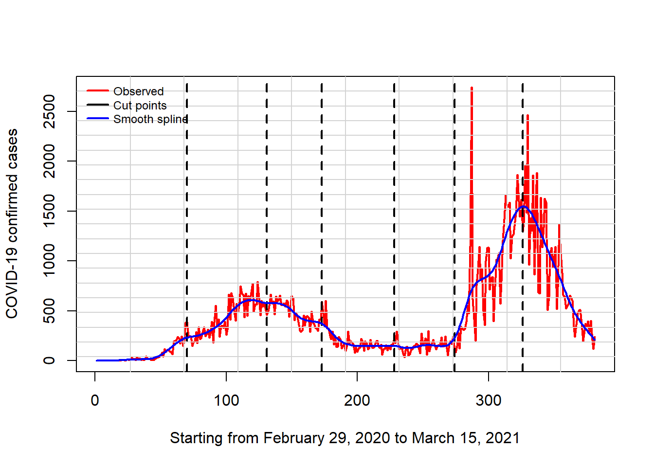
The above plot shows that as at March 15, 2021; Nigeria has gone through two waves and there were more cases of COVID-19 in the second wave.
plot(cumper$Per, main = " ",
     xlab = casesstarts, ylab = "Per Cent",
     ylim = c(-50,100),
     type = "l", lwd = 2, col="forestgreen")
grid(10,20,lty=1,lwd=1)
lines(cumper$Per, lty=1,lwd=2, col= "forestgreen")
lines(cumper$PerCum, lty=1,lwd=2, col= "orangered")
lines(log(cumper$DailyCase), lty=1,lwd=2, col= "magenta")
lines(cumper$LPer, lty=1,lwd=2, col= "brown")
lines(cumper$LPerCum, lty=1,lwd=2, col= "blue")
legend("topright",
       inset = c(0, 0, 0, 0),  bty = "n", x.intersp = 0.5,
       xjust = 0, yjust = 0,
       "topright", col = c("forestgreen", "orangered", "magenta", "brown", "blue"),
       c("Per cent of total cases","Percent of cummulative cases",
         "Daily cases, log transformed",
         "Difference from previsous rate",
         "Difference from previous cummulative rate"),
       lwd = 2, cex = 0.75, xpd = TRUE, horiz = FALSE)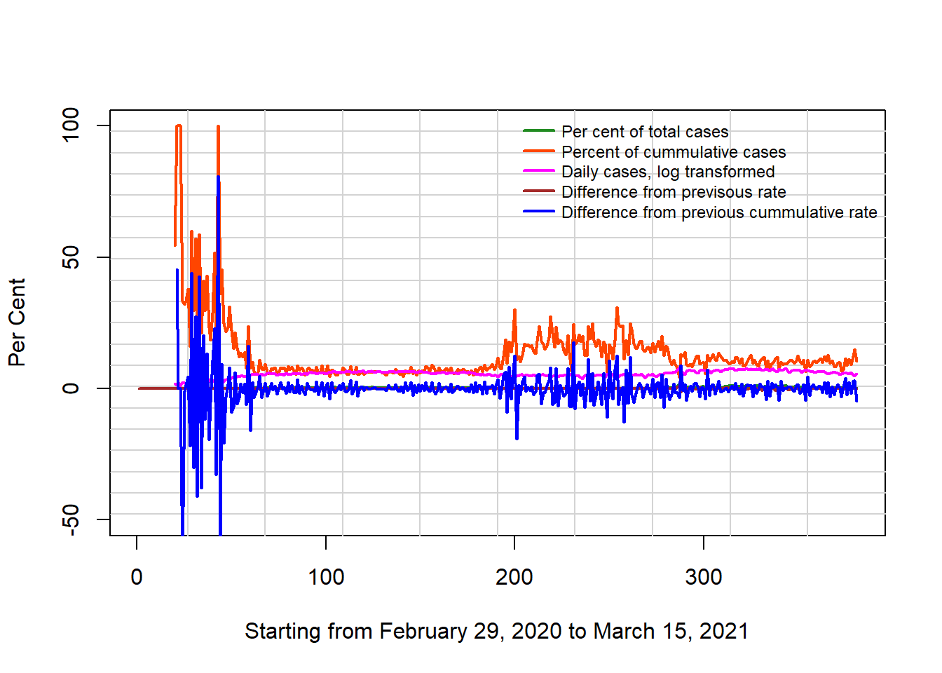
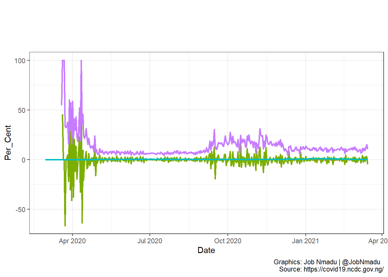
The above two visuals show the log transformation of the distribution and the difference from previous day. The plots were mage with plot and ggplot functions respectively.
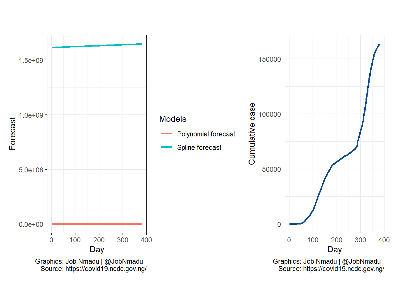
The plot on the right is the cumulative cases of COVID-19 recorded in Nigeria while on the left is the forecast using spline and polynomial models. The forecast is based on equal duation of the lenght of the data.