Introduction
The linear model still remains a reference point towards advanced modeling of some datasets as foundation for Machine Learning, Data Science and Artificial Intelligence in spite of some of her weaknesses. The major task in modeling is to compare various models before a selection is made for one or for advanced modeling. Often, some trial and error methods are used to decide which model to select. This is where this function is unique. It helps to estimate 14 different linear models and provide their coefficients in a formatted Table for quick comparison so that time and energy are saved. The interesting thing about this function is the simplicity, and it is a one line code. The different transformations are:
Linear model
Linear model with interactions
Semilog model
Growth model
Double Log model
Mixed-power model
Translog model
Quadratic model
Cubic model
Inverse of y model
Inverse of x model
Inverse of y & x model
Square root model
Cubic root model
In this blog, I share with you a function Linearsystems from Dyn4cast package which you can use in a very easy way to perform linear regression and or its various transformations. It is a one line code and easy to use. The usage is as follows:
Linearsystems(y, x, mod, limit, Test = NA)
y is the vector of the dependent variable.
x is the vector of the independent variables preferable in data.frame.
mod is the group of linear models to be estimated. It takes value from 0 to 6. 0 = EDA (correlation, summary tables, Visuals means); 1 = Linear systems, 2 = power models, 3 = polynomial models, 4 = root models, 5 = inverse models, 6 = all the 14 models.
limit is the number of variables to be included in the coefficients plots.
Test is the test data to be used to predict y. If not supplied, the fitted y is used hence may be identical with the fitted value.
With this one line of codes, in addition to the individual estimated models, the following are what you get:
Visual means of the numeric variable
Correlation plot
Significant plots of all the models estimated
Model Table
Machine Learning Metrics which is also a list of 47 performance and diagnostic statistic
Table of Marginal effects
Fitted plots long format
Fitted plots wide format
Prediction plots long format
Prediction plots wide format
Naive effects plots long format
Naive effects plots wide format
Summary of numeric variables
Summary of character variables
Let us dive into an awesome experience in machine learning!
Load library
library(Dyn4cast)Estimate without test data
y <- linearsystems$MKTcost
x <- select(linearsystems, -MKTcost)
Model1 <- Linearsystems(y, x, 6, 15)
Correlation matrix
Model1$`Correlation plot`$plot()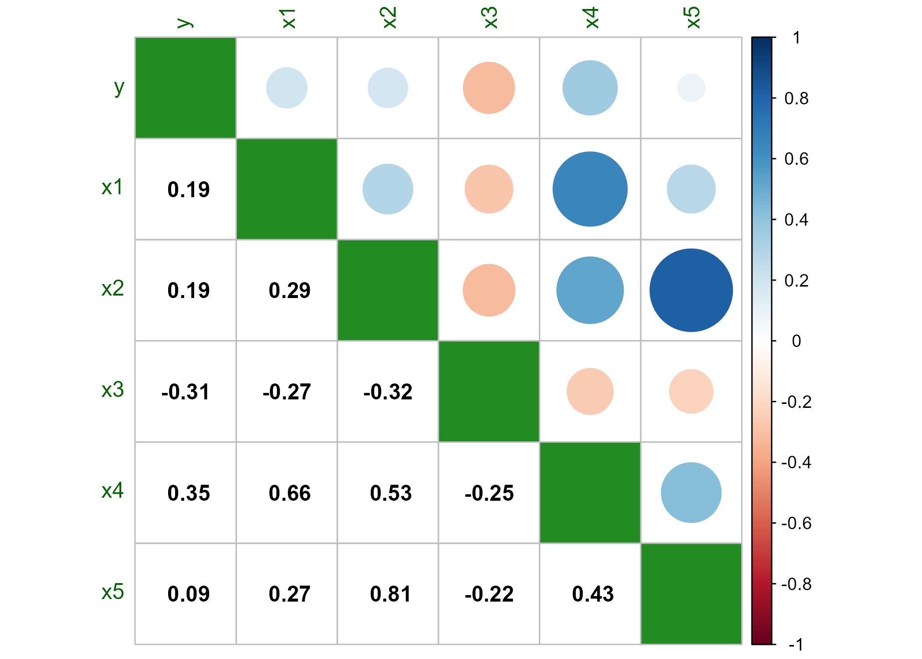
Model Table
Model1$`Model Table`| Linear | Cobb Douglas | Linlog | Loglin | Reciprocal in X | Reciprocal in Y | Double reciprocal | Quadratic | Square root | Cubic root | Cubic | Mixed-power | Translog | Linear with interaction | |
|---|---|---|---|---|---|---|---|---|---|---|---|---|---|---|
| (Intercept) | 1182.609 | 3.794** | 13.073* | 9.572*** | −0.935 | −0.291 | 1.496 | 10.051** | 12.979 | 14.920 | 7.998 | 12.093 | −914.830 | 178869.456 |
| (3733.003) | (1.278) | (4.964) | (2.514) | (2.459) | (0.289) | (1.129) | (3.638) | (12.254) | (18.472) | (12.105) | (16.289) | (1845.357) | (124754.685) | |
| Age | −26.698 | −0.446 | −1.729 | −0.042 | 7.921 | 0.005 | −3.596 | −0.043 | −0.035 | −0.036 | 0.088 | −0.037 | 261.741 | −5430.850 |
| (39.822) | (0.284) | (1.103) | (0.027) | (5.593) | (0.003) | (2.568) | (0.150) | (0.285) | (0.214) | (0.811) | (0.146) | (516.542) | (3483.580) | |
| Experience | 15.358 | −0.021 | −0.074 | 0.000 | 0.205 | 0.000 | −0.094 | −0.039 | 0.168 | 0.128 | −0.247 | 0.099 | 672.779 | −13992.660 |
| (119.313) | (0.244) | (0.950) | (0.080) | (1.228) | (0.009) | (0.564) | (0.368) | (0.589) | (0.433) | (0.985) | (0.316) | (798.885) | (16252.545) | |
| Years spent in formal education | 217.766 | −0.157 | −0.201 | 0.031 | 2.118 | 0.002 | −1.040 | −0.674 | 1.287 | 0.964 | −1.384 | 0.699 | 349.387 | −15364.578 |
| (196.683) | (0.436) | (1.693) | (0.132) | (2.493) | (0.015) | (1.144) | (0.631) | (1.013) | (0.750) | (2.634) | (0.541) | (740.038) | (11710.394) | |
| Household size | 317.218** | 0.269 | 1.423+ | 0.150+ | −0.930 | −0.010 | 0.375 | 0.015 | 0.274 | 0.235 | 0.728 | 0.207 | 338.839 | −18999.563 |
| (115.742) | (0.196) | (0.762) | (0.078) | (0.877) | (0.009) | (0.403) | (0.357) | (0.672) | (0.504) | (1.544) | (0.379) | (762.332) | (12326.813) | |
| Years as a cooperative member | −52.901 | −0.077 | −0.272 | −0.025 | 0.239 | 0.004 | −0.112 | −0.137 | 0.176 | 0.119 | −0.435 | 0.083 | 50.240 | −16929.904 |
| (130.234) | (0.247) | (0.960) | (0.088) | (1.183) | (0.010) | (0.543) | (0.357) | (0.602) | (0.448) | (1.183) | (0.332) | (849.055) | (17391.449) | |
| Marital statusMarried | 1842.879 | −0.247 | −0.589 | −0.555 | −0.130 | 0.135 | 0.064 | −0.225 | −0.137 | −0.137 | −0.176 | −0.133 | 0.105 | −2815.028 |
| (1715.980) | (0.277) | (1.075) | (1.156) | (0.134) | (0.133) | (0.062) | (1.290) | (1.312) | (1.314) | (1.420) | (1.314) | (0.327) | (3232.693) | |
| Marital statusSingle | 4142.944 | 0.153 | 1.932 | 0.396 | 0.570 | 0.122 | −0.209 | 0.117 | −0.396 | −0.851 | 2.167 | −0.081 | 0.666 | 4127.110 |
| (2619.350) | (0.552) | (2.144) | (1.764) | (0.748) | (0.203) | (0.343) | (2.101) | (5.621) | (8.373) | (4.340) | (4.742) | (2.819) | (6366.084) | |
| Marital statusWidowed | 2168.175 | −0.025 | 0.238 | 0.217 | −0.015 | 0.039 | 0.012 | 0.459 | 0.545 | 0.543 | 0.470 | 0.548 | 0.145 | −1061.522 |
| (1560.281) | (0.262) | (1.016) | (1.051) | (0.133) | (0.121) | (0.061) | (1.185) | (1.178) | (1.175) | (1.277) | (1.174) | (0.287) | (3056.615) | |
| Main OccupationMarketing of Agricultural produce | 696.759 | −0.089 | −0.279 | −0.194 | −0.059 | 0.032 | 0.028 | −0.163 | −0.163 | −0.162 | −0.132 | −0.162 | −0.029 | 871.619 |
| (988.961) | (0.172) | (0.667) | (0.666) | (0.089) | (0.077) | (0.041) | (0.686) | (0.684) | (0.684) | (0.711) | (0.684) | (0.125) | (1136.352) | |
| Main OccupationSale of provision | 974.225 | 0.010 | 0.150 | 0.182 | −0.001 | 0.002 | 0.002 | 0.158 | 0.210 | 0.217 | 0.295 | 0.221 | 0.039 | 705.656 |
| (1227.830) | (0.214) | (0.832) | (0.827) | (0.112) | (0.095) | (0.052) | (0.871) | (0.862) | (0.861) | (0.946) | (0.861) | (0.170) | (1546.785) | |
| Level of educationNon-formal | −4535.272 | −0.045 | −1.255 | −2.159 | 1.732 | 0.178 | −0.859 | 2.457 | 13.394 | 20.708 | 4.919 | 12.420 | 1.798 | −7893.322 |
| (3088.096) | (1.182) | (4.591) | (2.080) | (2.312) | (0.239) | (1.061) | (4.227) | (12.301) | (17.922) | (10.034) | (11.352) | (4.440) | (9121.469) | |
| Level of educationPrimary | −1891.589 | 0.094 | −0.460 | −1.164 | 1.748 | 0.102 | −0.862 | 2.917 | 13.843 | 21.153 | 5.386 | 12.866 | 1.871 | −4970.197 |
| (1948.345) | (0.964) | (3.744) | (1.312) | (2.202) | (0.151) | (1.011) | (3.489) | (11.776) | (17.436) | (9.624) | (10.828) | (4.372) | (8139.493) | |
| Level of educationSecondary | −4243.879 | 0.336 | 0.018 | −0.927 | 1.943 | −0.004 | −0.958 | 3.913 | 14.780 | 22.087 | 6.378 | 13.791 | 2.017 | −7558.975 |
| (2878.842) | (1.175) | (4.566) | (1.939) | (2.317) | (0.223) | (1.064) | (4.360) | (12.447) | (18.071) | (9.725) | (11.481) | (4.474) | (9144.744) | |
| Level of educationTertiary | −5416.211 | 0.325 | −0.166 | −1.233 | 1.950 | 0.006 | −0.963 | 3.383 | 14.186 | 21.490 | 5.702 | 13.189 | 1.937 | −9340.187 |
| (3356.079) | (1.248) | (4.849) | (2.261) | (2.345) | (0.260) | (1.077) | (4.393) | (12.329) | (17.932) | (9.464) | (11.364) | (4.432) | (9561.933) | |
| IAge | 0.000 | −0.049 | −0.098 | −0.003 | −0.048 | −0.174 | ||||||||
| (0.002) | (3.637) | (7.544) | (0.020) | (5.969) | (1.124) | |||||||||
| IExperience | 0.003 | −0.975 | −1.578 | 0.022 | −0.932 | 0.881 | ||||||||
| (0.015) | (3.916) | (6.370) | (0.085) | (3.676) | (1.112) | |||||||||
| IYears spent in formal education | 0.027 | −8.762 | −14.761 | 0.088 | −8.700 | 0.409 | ||||||||
| (0.024) | (7.050) | (11.744) | (0.227) | (6.884) | (0.677) | |||||||||
| IHousehold size | 0.006 | −0.793 | −1.200 | −0.069 | −0.644 | −0.134 | ||||||||
| (0.018) | (3.992) | (6.394) | (0.164) | (3.638) | (0.571) | |||||||||
| IYears as a cooperative member | 0.006 | −1.194 | −1.801 | 0.035 | −1.017 | 1.074 | ||||||||
| (0.015) | (3.870) | (6.291) | (0.109) | (3.629) | (1.178) | |||||||||
| ICAge | 0.000 | |||||||||||||
| (0.000) | ||||||||||||||
| ICExperience | −0.001 | |||||||||||||
| (0.002) | ||||||||||||||
| ICYears spent in formal education | −0.002 | |||||||||||||
| (0.006) | ||||||||||||||
| ICHousehold size | 0.002 | |||||||||||||
| (0.005) | ||||||||||||||
| ICYears as a cooperative member | −0.001 | |||||||||||||
| (0.003) | ||||||||||||||
| Age × Experience | −187.488 | 413.060 | ||||||||||||
| (222.702) | (421.287) | |||||||||||||
| Age × Years spent in formal education | −99.604 | 487.222 | ||||||||||||
| (208.652) | (333.733) | |||||||||||||
| Experience × Years spent in formal education | −260.899 | 1263.591 | ||||||||||||
| (316.027) | (1423.802) | |||||||||||||
| Age × Household size | −97.341 | 626.189+ | ||||||||||||
| (213.777) | (326.989) | |||||||||||||
| Experience × Household size | −256.864 | 1524.101 | ||||||||||||
| (321.486) | (1450.023) | |||||||||||||
| Years spent in formal education × Household size | −129.986 | 1885.469 | ||||||||||||
| (307.538) | (1237.124) | |||||||||||||
| Age × Years as a cooperative member | −20.388 | 567.013 | ||||||||||||
| (237.791) | (470.536) | |||||||||||||
| Experience × Years as a cooperative member | −146.606 | 1314.591 | ||||||||||||
| (322.411) | (1078.651) | |||||||||||||
| Years spent in formal education × Years as a cooperative member | −19.775 | 1402.282 | ||||||||||||
| (339.431) | (1512.580) | |||||||||||||
| Household size × Years as a cooperative member | −9.780 | 1598.233 | ||||||||||||
| (349.012) | (1616.021) | |||||||||||||
| Age × Experience × Years spent in formal education | 72.621 | −38.214 | ||||||||||||
| (88.449) | (38.386) | |||||||||||||
| Age × Experience × Household size | 71.786 | −45.862 | ||||||||||||
| (89.607) | (36.700) | |||||||||||||
| Age × Years spent in formal education × Household size | 37.224 | −59.358+ | ||||||||||||
| (86.574) | (35.423) | |||||||||||||
| Experience × Years spent in formal education × Household size | 99.695 | −141.079 | ||||||||||||
| (127.942) | (135.348) | |||||||||||||
| Age × Experience × Years as a cooperative member | 41.773 | −41.293 | ||||||||||||
| (90.451) | (29.463) | |||||||||||||
| Age × Years spent in formal education × Years as a cooperative member | 7.558 | −45.465 | ||||||||||||
| (95.569) | (43.009) | |||||||||||||
| Experience × Years spent in formal education × Years as a cooperative member | 56.856 | −106.971 | ||||||||||||
| (128.179) | (96.548) | |||||||||||||
| Age × Household size × Years as a cooperative member | 5.684 | −57.279 | ||||||||||||
| (97.274) | (41.653) | |||||||||||||
| Experience × Household size × Years as a cooperative member | 53.271 | −124.988 | ||||||||||||
| (130.612) | (94.861) | |||||||||||||
| Years spent in formal education × Household size × Years as a cooperative member | 3.965 | −148.608 | ||||||||||||
| (139.964) | (139.454) | |||||||||||||
| Age × Experience × Years spent in formal education × Household size | −27.844 | 4.331 | ||||||||||||
| (35.809) | (3.616) | |||||||||||||
| Age × Experience × Years spent in formal education × Years as a cooperative member | −16.311 | 3.364 | ||||||||||||
| (36.096) | (2.695) | |||||||||||||
| Age × Experience × Household size × Years as a cooperative member | −15.558 | 4.083 | ||||||||||||
| (36.514) | (2.543) | |||||||||||||
| Age × Years spent in formal education × Household size × Years as a cooperative member | −2.115 | 5.009 | ||||||||||||
| (39.255) | (3.834) | |||||||||||||
| Experience × Years spent in formal education × Household size × Years as a cooperative member | −21.016 | 10.938 | ||||||||||||
| (51.999) | (8.733) | |||||||||||||
| Age × Experience × Years spent in formal education × Household size × Years as a cooperative member | 6.104 | −0.356 | ||||||||||||
| (14.611) | (0.241) | |||||||||||||
| Num.Obs. | 100 | 100 | 100 | 100 | 100 | 100 | 100 | 100 | 100 | 100 | 100 | 100 | 100 | 100 |
| R2 | 0.269 | 0.134 | 0.139 | 0.144 | 0.136 | 0.144 | 0.141 | 0.166 | 0.168 | 0.168 | 0.173 | 0.168 | 0.248 | 0.471 |
| R2 Adj. | 0.149 | −0.008 | −0.003 | 0.003 | −0.006 | 0.003 | −0.001 | −0.032 | −0.030 | −0.030 | −0.092 | −0.030 | −0.379 | 0.112 |
| AIC | 1867.6 | 136.2 | 407.6 | 407.0 | 6.6 | −25.8 | −149.1 | 414.4 | 414.2 | 414.2 | 423.6 | 414.2 | 54.8 | 1887.3 |
| BIC | 1909.3 | 177.9 | 449.3 | 448.7 | 48.3 | 15.9 | −107.4 | 469.1 | 468.9 | 468.9 | 491.3 | 468.9 | 177.2 | 1996.7 |
| Log.Lik. | −917.806 | −52.086 | −187.788 | −187.515 | 12.708 | 28.878 | 90.564 | −186.183 | −186.107 | −186.112 | −185.782 | −186.105 | 19.615 | −901.648 |
| F | 2.235 | 0.941 | 0.982 | 1.021 | 0.959 | 1.018 | 0.996 | 0.841 | 0.848 | 0.848 | 0.654 | 0.849 | 0.395 | |
| RMSE | 2342.84 | 0.41 | 1.58 | 1.58 | 0.21 | 0.18 | 0.10 | 1.56 | 1.56 | 1.56 | 1.55 | 1.56 | 0.20 | 1993.28 |
| + p < 0.1, * p < 0.05, ** p < 0.01, *** p < 0.001 |
Significant plot
Individual model has one
Model1$`Significant plot of Double Log`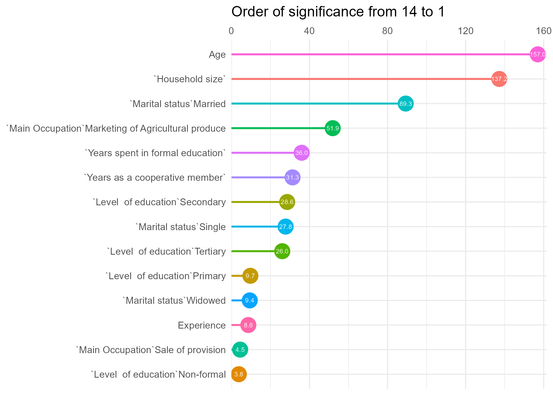
Fitted estimates
Model1$`Fitted plots wide format`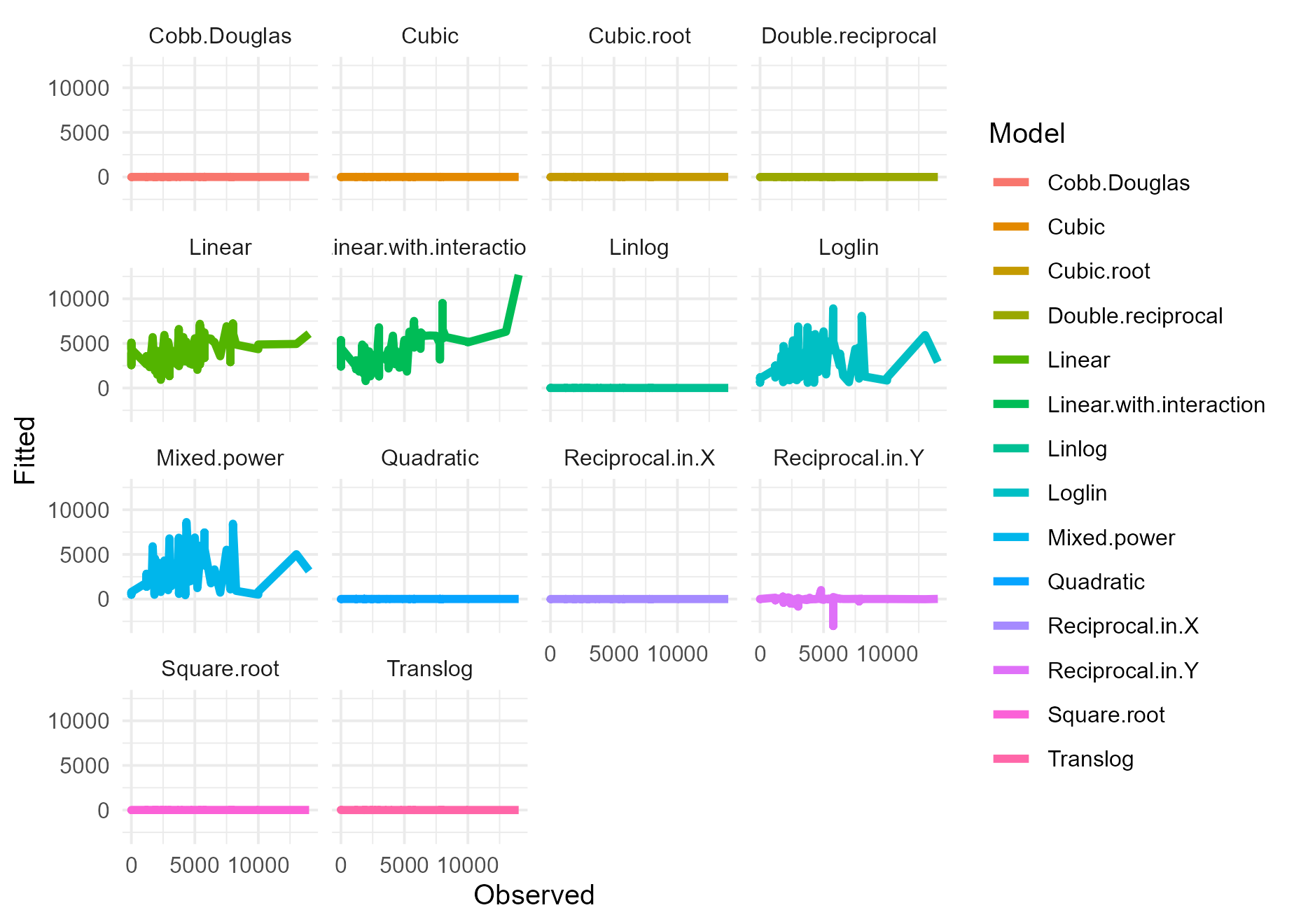
Marginal effects
Model1$`Tables of marginal effects`[[1]]| Linear | Linear with interaction | |
|---|---|---|
| Age dY/dX | −26.698 | −81.589 |
| (39.826) | (3168.661) | |
| Experience dY/dX | 15.358 | −2.022 |
| (119.309) | (1773.827) | |
| Household size dY/dX | 317.218*** | 429.647*** |
| (0.041) | (0.998) | |
| Level of education Non-formal - Illiterate | −4535.272 | −7893.322*** |
| (0.001) | ||
| Level of education Primary - Illiterate | −1891.589 | −4970.197*** |
| (0.001) | ||
| Level of education Secondary - Illiterate | −4243.879 | −7558.975*** |
| (0.001) | ||
| Level of education Tertiary - Illiterate | −5416.211 | −9340.187*** |
| (0.001) | ||
| Main Occupation Marketing of Agricultural produce - Civil Servant | 696.759 | 871.619*** |
| (0.001) | ||
| Main Occupation Sale of provision - Civil Servant | 974.225 | 705.656*** |
| (0.001) | ||
| Marital status Married - Divorced | 1842.879*** | −2815.028*** |
| (0.000) | (0.001) | |
| Marital status Single - Divorced | 4142.944 | 4127.110*** |
| (0.001) | ||
| Marital status Widowed - Divorced | 2168.175 | −1061.522*** |
| (0.000) | ||
| Years as a cooperative member dY/dX | −52.901*** | −32.928*** |
| (0.019) | (0.439) | |
| Years spent in formal education dY/dX | 217.766*** | 263.233*** |
| (0.054) | (1.064) | |
| Num.Obs. | 100 | 100 |
| R2 | 0.269 | 0.471 |
| R2 Adj. | 0.149 | 0.112 |
| AIC | 1867.6 | 1887.3 |
| BIC | 1909.3 | 1996.7 |
| Log.Lik. | −917.806 | −901.648 |
| F | 2.235 | |
| RMSE | 2342.84 | 1993.28 |
| + p < 0.1, * p < 0.05, ** p < 0.01, *** p < 0.001 |
Naive effects
Model1$`Naive effects plots long format`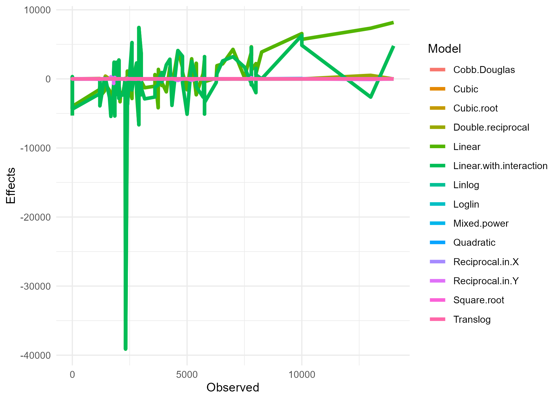
Estimation with test data
x <- sampling[, -1]
y <- sampling$qOutput
Data <- cbind(y, x)
sampling <- sample(1:nrow(Data), 0.8 * nrow(Data)) # 80% of data is sampled for training the model
train <- Data[sampling, ]
Test <- Data[-sampling, ] # 20% of data is reserved for testing (predicting) the model
y <- train$y
x <- train[, -1]
mod <- 4
Model2 <- Linearsystems(y, x, 4, 15, Test)
Model2$`Model Table`| Linear | Square root | Cubic root | |
|---|---|---|---|
| (Intercept) | −260.945** | 7.664*** | 6.490*** |
| (96.670) | (0.475) | (0.670) | |
| qLabor | −84.260 | 1.453 | 0.421 |
| (73.512) | (1.015) | (0.759) | |
| land | 25.807*** | −0.048*** | −0.039*** |
| (1.555) | (0.008) | (0.006) | |
| qVarInput | 1.220*** | 0.003 | 0.003+ |
| (0.075) | (0.002) | (0.001) | |
| time | 20.992*** | −0.006* | 0.001 |
| (1.436) | (0.002) | (0.002) | |
| IqLabor | −3.778 | −2.034 | |
| (2.410) | (2.851) | ||
| Iland | 0.753*** | 1.726*** | |
| (0.080) | (0.159) | ||
| IqVarInput | −0.108 | −0.436 | |
| (0.091) | (0.306) | ||
| Itime | 0.126*** | 0.179*** | |
| (0.008) | (0.014) | ||
| Num.Obs. | 160 | 160 | 160 |
| R2 | 1.000 | 1.000 | 1.000 |
| R2 Adj. | 1.000 | 1.000 | 1.000 |
| AIC | 1127.7 | −1130.2 | −1127.6 |
| BIC | 1146.2 | −1099.5 | −1096.9 |
| Log.Lik. | −557.874 | 575.109 | 573.808 |
| F | 5059140.593 | 157990.105 | 155442.975 |
| RMSE | 7.91 | 0.01 | 0.01 |
| + p < 0.1, * p < 0.05, ** p < 0.01, *** p < 0.001 |
Model Table
Model2$`Table of Marginal effects`| Linear | Square root | Cubic root | |
|---|---|---|---|
| land | 25.807*** | −0.048*** | −0.039*** |
| (1.555) | (0.008) | (0.006) | |
| qLabor | −84.260 | 1.453 | 0.421 |
| (73.495) | (1.015) | (0.759) | |
| qVarInput | 1.220*** | 0.003 | 0.003+ |
| (0.075) | (0.002) | (0.001) | |
| time | 20.992*** | −0.006** | 0.001 |
| (1.436) | (0.002) | (0.002) | |
| Iland | 0.753*** | 1.726*** | |
| (0.080) | (0.159) | ||
| IqLabor | −3.778 | −2.034 | |
| (2.410) | (2.850) | ||
| IqVarInput | −0.108 | −0.436 | |
| (0.091) | (0.306) | ||
| Itime | 0.126*** | 0.179*** | |
| (0.008) | (0.014) | ||
| Num.Obs. | 160 | 160 | 160 |
| R2 | 1.000 | 1.000 | 1.000 |
| R2 Adj. | 1.000 | 1.000 | 1.000 |
| AIC | 1127.7 | −1130.2 | −1127.6 |
| BIC | 1146.2 | −1099.5 | −1096.9 |
| Log.Lik. | −557.874 | 575.109 | 573.808 |
| F | 5059140.593 | 157990.105 | 155442.975 |
| RMSE | 7.91 | 0.01 | 0.01 |
| + p < 0.1, * p < 0.05, ** p < 0.01, *** p < 0.001 |
Visualise means of the numeric variables
Model2$`Visual means of the numeric variable`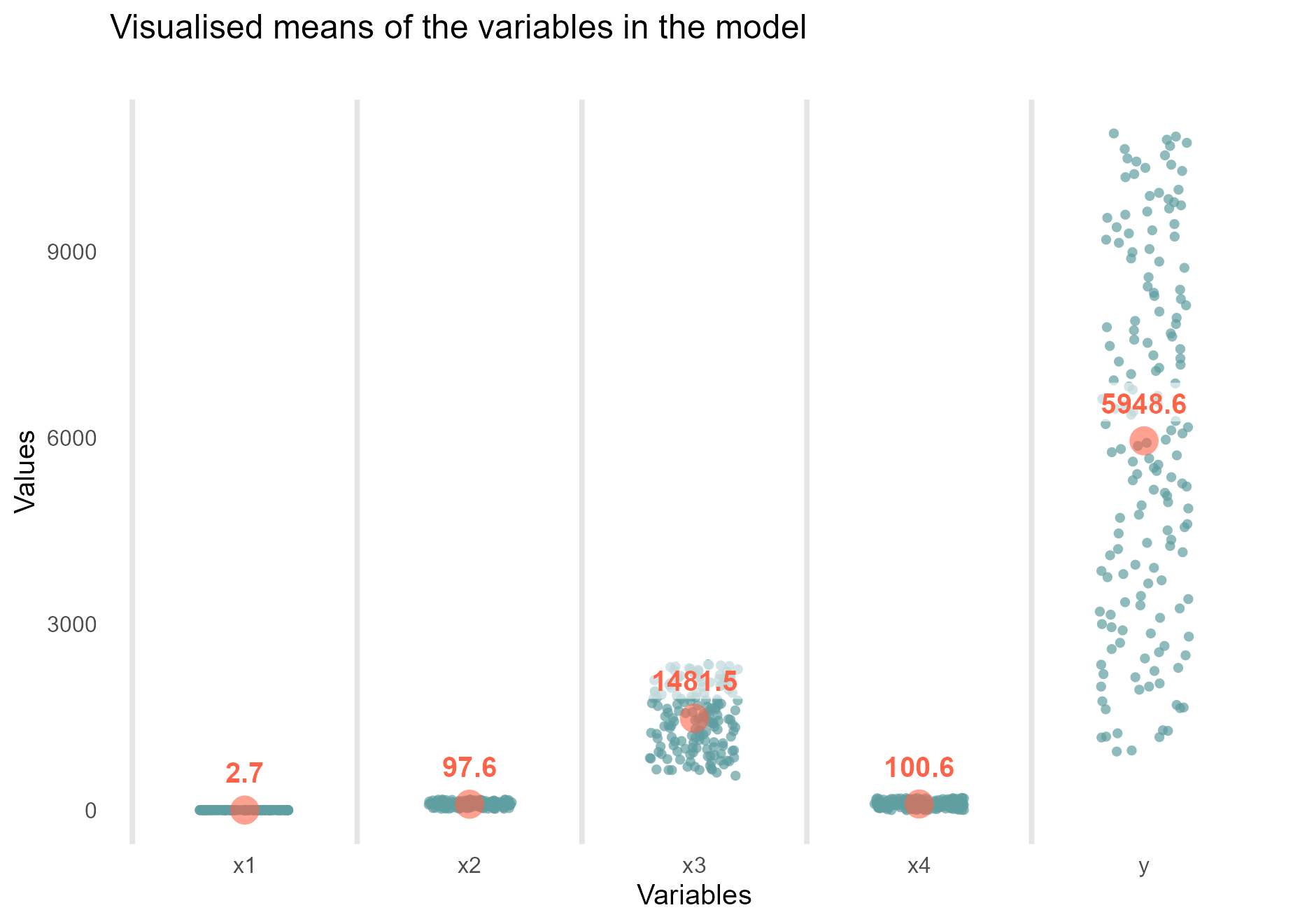
Fitted estimates
Model2$`Fitted plots long format`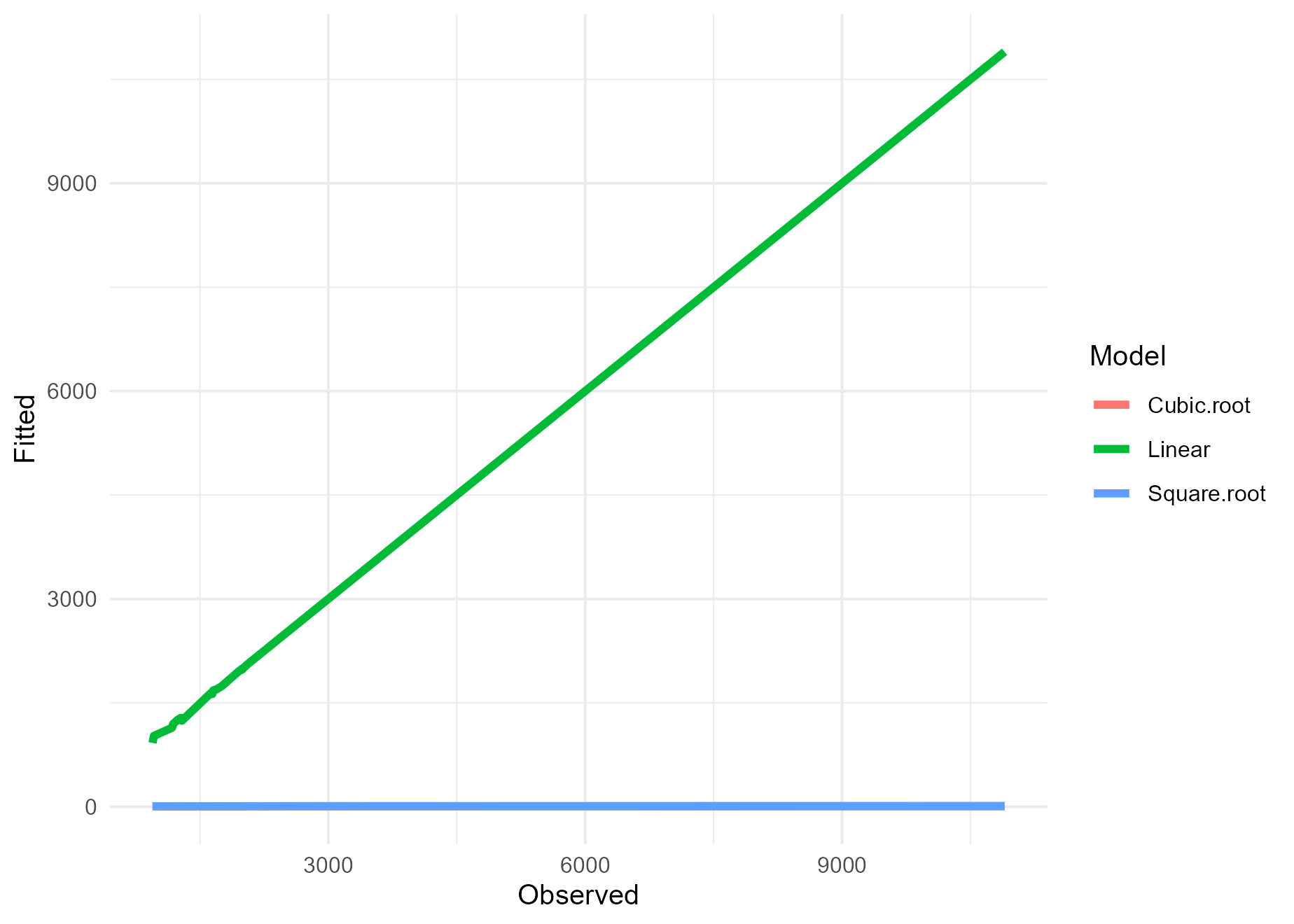
Predicted
Model2$`Prediction plots long format`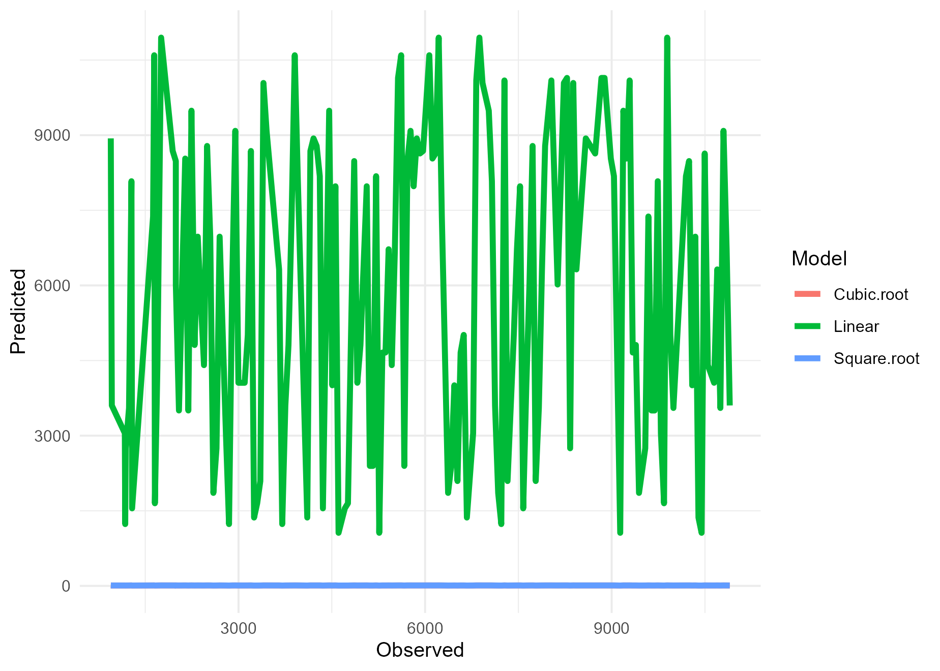
Significant plot
Model2$`Significant plot of Square root`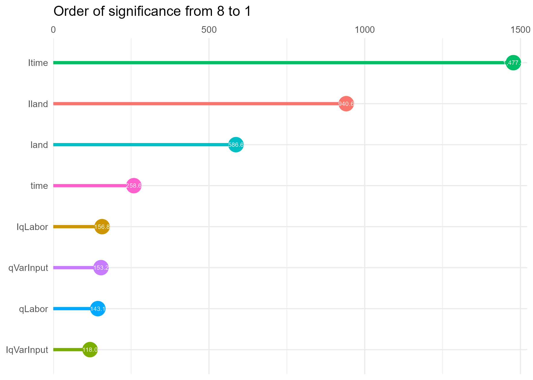
Performance and Diagnostic values
Model2$`Machine Learning Metrics`| Name | Linear | Square.root | Cubic.root |
|---|---|---|---|
| Absolute Error | 380 | 0.33 | 0.35 |
| Absolute Percent Error | 0.27 | 0.045 | 0.047 |
| Accuracy | 0 | 0 | 0 |
| Adjusted R Square | 1 | 1 | 1 |
| Akaike’s Information Criterion AIC | 1100 | -1100 | -1100 |
| Allen’s Prediction Sum-Of-Squares (PRESS, P-Square) | 0 | 0 | 0 |
| Area under the ROC curve (AUC) | 0 | 0 | 0 |
| Average Precision at k | 0 | 0 | 0 |
| Bias | 5e-15 | 1.1e-17 | 7.2e-17 |
| Brier score | 60 | 4e-05 | 4e-05 |
| Classification Error | 1 | 1 | 1 |
| F1 Score | 0 | 0 | 0 |
| fScore | 0 | 0 | 0 |
| GINI Coefficient | 1 | 1 | 1 |
| kappa statistic | 0 | 0 | 0 |
| Log Loss | Inf | Inf | Inf |
| Mallow’s cp | 5 | 9 | 9 |
| Matthews Correlation Coefficient | 0 | 0 | 0 |
| Mean Log Loss | -210000 | -260 | -260 |
| Mean Absolute Error | 2.4 | 0.0021 | 0.0022 |
| Mean Absolute Percent Error | 0.0017 | 0.00028 | 0.00029 |
| Mean Average Precision at k | 0 | 0 | 0 |
| Mean Absolute Scaled Error | 0.00072 | 0.0031 | 0.0032 |
| Median Absolute Error | 0.55 | 0.00053 | 0.00064 |
| Mean Squared Error | 63 | 4.4e-05 | 4.5e-05 |
| Mean Squared Log Error | 4.9e-05 | 6.9e-07 | 7e-07 |
| Model turning point error | 0 | 0 | 0 |
| Negative Predictive Value | 0 | 0 | 0 |
| Percent Bias | 5.6e-05 | -8.7e-07 | -8.9e-07 |
| Positive Predictive Value | 0 | 0 | 0 |
| Precision | 0 | 0 | 0 |
| R Square | 1 | 1 | 1 |
| Relative Absolute Error | 0.00097 | 0.0042 | 0.0044 |
| Recall | NaN | NaN | NaN |
| Root Mean Squared Error | 7.9 | 0.0066 | 0.0067 |
| Root Mean Squared Log Error | 0.007 | 0.00083 | 0.00083 |
| Root Relative Squared Error | 0.0028 | 0.011 | 0.011 |
| Relative Squared Error | 7.7e-06 | 0.00012 | 0.00012 |
| Schwarz’s Bayesian criterion BIC | 1100 | -1100 | -1100 |
| Sensitivity | 0 | 0 | 0 |
| specificity | 0 | 0 | 0 |
| Squared Error | 10000 | 0.0071 | 0.0072 |
| Squared Log Error | 0.0078 | 0.00011 | 0.00011 |
| Symmetric Mean Absolute Percentage Error | 0.0017 | 0.00028 | 0.00029 |
| Sum of Squared Errors | 10000 | 0.0071 | 0.0072 |
| True negative rate | 0 | 0 | 0 |
| True positive rate | 0 | 0 | 0 |
Welcome to easy machine learning and models estimation!