Introduction
This blog is about two new functions, Model_factors and garrett_ranking that have been added to the Dyn4cast package. The two functions provides means for gaining deeper insights into the meaning behind Likert-type variables collected from respondents. Garrett ranking provides the ranks of the observations of the variables based on the level of seriousness attached to it by the respondents. On the other hand, Model factors determines and retrieve the latent factors inherent in such data which now becomes continuous data. The factors or data frame retrieved from the variables can be used in other analysis like regression and machine learning.
The two functions are part of factor analysis, essentially, exploratory factor analysis (EFA), used to unravel the underlying structure of the observed variables. The analysis also helps to reduce the complex structure by determining a smaller number of latent factors that sufficiently represent the variation in the observed variables. With EFA, no prior knowledge or hypothesis about the number or nature of the factors is assumed. These are great tools to help tell the story behind your data. The data used for Model_factors is prepared using fa.parallel and fa functions in the psych package. The interesting thing about these functions are their simplicity, and we still maintain the one line code technique.
The basic usage of the codes are:
garrett_ranking(data, num_rank, ranking = NULL, m_rank = c(2:15))
Data The data for the Garrett Ranking.
num_rank number of ranks applied to the data. If the data is a five-point Likert-type data, then number of ranks is 5.
Ranking A vector of list representing the ranks applied to the data. If not available, positional ranks are applied.
m_rank scope of ranking (2-15).
Model_factors(data = dat, DATA = Data)
data R object obtained from EFA using the fa function in psych package
DATA data.frame of the raw data used to obtain data object.
Let us go!
Load library
library(Dyn4cast)Garrett Ranking
ranking is supplied
garrett_data <- data.frame(garrett_data)
ranking <- c(
  "Serious constraint", "Constraint",
  "Not certain it is a constraint", "Not a constraint",
  "Not a serious constraint"
)

garrett_ranking(garrett_data, 5, ranking)
$`Garrett value`
# A tibble: 5 × 4
Number `Garrett point` `Garrett index` `Garrett value`
<dbl> <dbl> <dbl> <dbl>
1 1 3.33 15 85
2 2 10 25 75
3 3 16.7 31 69
4 4 23.3 36 64
5 5 30 40 60
$`Garrett ranked data`
S/No Description Serious constraint Constraint
1 2 S2 5 3
2 9 S9 7 6
3 15 S15 7 6
4 5 S5 10 2
5 11 S11 10 2
6 4 S4 4 4
7 10 S10 4 4
8 3 S3 1 2
9 1 S1 0 0
10 6 S6 0 4
11 12 S12 0 4
12 7 S7 0 2
13 13 S13 0 2
14 8 S8 0 0
15 14 S14 0 0
Not certain it is a constraint Not a constraint Not a serious constraint
1 2 2 1
2 0 5 1
3 0 5 1
4 8 5 0
5 8 5 0
6 6 7 3
7 6 7 3
8 5 5 1
9 2 1 0
10 6 5 6
11 6 5 6
12 0 2 2
13 0 2 2
14 5 2 17
15 5 2 17
Total Mean Total Garrett Score Mean Garrett score Total Item score
1 13 8.172414 976 75.07692 48
2 19 4.517241 1425 75.00000 70
3 19 4.517241 1425 75.00000 70
4 25 3.413793 1872 74.88000 92
5 25 3.413793 1872 74.88000 92
6 24 3.310345 1682 70.08333 71
7 24 3.310345 1682 70.08333 71
8 14 5.965517 960 68.57143 39
9 3 14.758621 202 67.33333 8
10 21 3.965517 1394 66.38095 50
11 21 3.965517 1394 66.38095 50
12 6 7.034483 398 66.33333 14
13 6 7.034483 398 66.33333 14
14 24 1.862069 1493 62.20833 36
15 24 1.862069 1493 62.20833 36
Relative importance index Rank
1 0.33103448 1
2 0.48275862 2
3 0.48275862 3
4 0.63448276 4
5 0.63448276 5
6 0.48965517 6
7 0.48965517 7
8 0.26896552 8
9 0.05517241 9
10 0.34482759 10
11 0.34482759 11
12 0.09655172 12
13 0.09655172 13
14 0.24827586 14
15 0.24827586 15
$RII
V1 V2 V3 V4 V5
1 0 0 6 2 0
2 25 12 6 4 1
3 5 8 15 10 1
4 20 16 18 14 3
5 50 8 24 10 0
6 0 16 18 10 6
7 0 8 0 4 2
8 0 0 15 4 17
9 35 24 0 10 1
10 20 16 18 14 3
11 50 8 24 10 0
12 0 16 18 10 6
13 0 8 0 4 2
14 0 0 15 4 17
15 35 24 0 10 1ranking not supplied
garrett_ranking(garrett_data, 5)$`Garrett value`
# A tibble: 5 × 4
Number `Garrett point` `Garrett index` `Garrett value`
<dbl> <dbl> <dbl> <dbl>
1 1 3.33 15 85
2 2 10 25 75
3 3 16.7 31 69
4 4 23.3 36 64
5 5 30 40 60
$`Garrett ranked data`
S/No Description 1st Rank 2nd Rank 3rd Rank 4th Rank 5th Rank Total
1 2 S2 5 3 2 2 1 13
2 9 S9 7 6 0 5 1 19
3 15 S15 7 6 0 5 1 19
4 5 S5 10 2 8 5 0 25
5 11 S11 10 2 8 5 0 25
6 4 S4 4 4 6 7 3 24
7 10 S10 4 4 6 7 3 24
8 3 S3 1 2 5 5 1 14
9 1 S1 0 0 2 1 0 3
10 6 S6 0 4 6 5 6 21
11 12 S12 0 4 6 5 6 21
12 7 S7 0 2 0 2 2 6
13 13 S13 0 2 0 2 2 6
14 8 S8 0 0 5 2 17 24
15 14 S14 0 0 5 2 17 24
Mean Total Garrett Score Mean Garrett score Total Item score
1 8.172414 976 75.07692 48
2 4.517241 1425 75.00000 70
3 4.517241 1425 75.00000 70
4 3.413793 1872 74.88000 92
5 3.413793 1872 74.88000 92
6 3.310345 1682 70.08333 71
7 3.310345 1682 70.08333 71
8 5.965517 960 68.57143 39
9 14.758621 202 67.33333 8
10 3.965517 1394 66.38095 50
11 3.965517 1394 66.38095 50
12 7.034483 398 66.33333 14
13 7.034483 398 66.33333 14
14 1.862069 1493 62.20833 36
15 1.862069 1493 62.20833 36
Relative importance index Rank
1 0.33103448 1
2 0.48275862 2
3 0.48275862 3
4 0.63448276 4
5 0.63448276 5
6 0.48965517 6
7 0.48965517 7
8 0.26896552 8
9 0.05517241 9
10 0.34482759 10
11 0.34482759 11
12 0.09655172 12
13 0.09655172 13
14 0.24827586 14
15 0.24827586 15
$RII
V1 V2 V3 V4 V5
1 0 0 6 2 0
2 25 12 6 4 1
3 5 8 15 10 1
4 20 16 18 14 3
5 50 8 24 10 0
6 0 16 18 10 6
7 0 8 0 4 2
8 0 0 15 4 17
9 35 24 0 10 1
10 20 16 18 14 3
11 50 8 24 10 0
12 0 16 18 10 6
13 0 8 0 4 2
14 0 0 15 4 17
15 35 24 0 10 1you can rank subset of the data
garrett_ranking(garrett_data, 8)$`Garrett value`
# A tibble: 8 × 4
Number `Garrett point` `Garrett index` `Garrett value`
<dbl> <dbl> <dbl> <dbl>
1 1 3.33 15 85
2 2 10 25 75
3 3 16.7 31 69
4 4 23.3 36 64
5 5 30 40 60
6 6 36.7 43 57
7 7 43.3 47 53
8 8 50 50 50
$`Garrett ranked data`
S/No Description 1st Rank 2nd Rank 3rd Rank 4th Rank 5th Rank 6th Rank
1 7 S7 4 2 2 0 2 0
2 13 S13 4 2 2 0 2 0
3 2 S2 2 0 2 5 3 2
4 9 S9 0 4 4 7 6 0
5 15 S15 0 4 4 7 6 0
6 3 S3 1 3 4 1 2 5
7 5 S5 0 1 0 10 2 8
8 11 S11 0 1 0 10 2 8
9 4 S4 0 1 3 4 4 6
10 10 S10 0 1 3 4 4 6
11 6 S6 0 1 1 0 4 6
12 12 S12 0 1 1 0 4 6
13 1 S1 0 0 0 0 0 2
14 8 S8 1 0 0 0 0 5
15 14 S14 1 0 0 0 0 5
7th Rank 8th Rank Total Mean Total Garrett Score Mean Garrett score
1 2 2 14 7.034483 954 68.14286
2 2 2 14 7.034483 954 68.14286
3 2 1 17 8.172414 1078 63.41176
4 5 1 27 4.517241 1699 62.92593
5 5 1 27 4.517241 1699 62.92593
6 5 1 22 5.965517 1370 62.27273
7 5 0 26 3.413793 1556 59.84615
8 5 0 26 3.413793 1556 59.84615
9 7 3 28 3.310345 1641 58.60714
10 7 3 28 3.310345 1641 58.60714
11 5 6 23 3.965517 1291 56.13043
12 5 6 23 3.965517 1291 56.13043
13 1 0 3 14.758621 167 55.66667
14 2 17 25 1.862069 1326 53.04000
15 2 17 25 1.862069 1326 53.04000
Total Item score Relative importance index Rank
1 72 0.31034483 1
2 72 0.31034483 2
3 76 0.32758621 3
4 122 0.52586207 4
5 122 0.52586207 5
6 92 0.39655172 6
7 99 0.42672414 7
8 99 0.42672414 8
9 96 0.41379310 9
10 96 0.41379310 10
11 63 0.27155172 11
12 63 0.27155172 12
13 8 0.03448276 13
14 44 0.18965517 14
15 44 0.18965517 15
$RII
V1 V2 V3 V4 V5 V6 V7 V8
1 0 0 0 0 0 6 2 0
2 16 0 12 25 12 6 4 1
3 8 21 24 5 8 15 10 1
4 0 7 18 20 16 18 14 3
5 0 7 0 50 8 24 10 0
6 0 7 6 0 16 18 10 6
7 32 14 12 0 8 0 4 2
8 8 0 0 0 0 15 4 17
9 0 28 24 35 24 0 10 1
10 0 7 18 20 16 18 14 3
11 0 7 0 50 8 24 10 0
12 0 7 6 0 16 18 10 6
13 32 14 12 0 8 0 4 2
14 8 0 0 0 0 15 4 17
15 0 28 24 35 24 0 10 1garrett_ranking(garrett_data, 4)$`Garrett value`
# A tibble: 4 × 4
Number `Garrett point` `Garrett index` `Garrett value`
<dbl> <dbl> <dbl> <dbl>
1 1 3.33 15 85
2 2 10 25 75
3 3 16.7 31 69
4 4 23.3 36 64
$`Garrett ranked data`
S/No Description 1st Rank 2nd Rank 3rd Rank 4th Rank Total Mean
1 9 S9 6 0 5 1 12 4.517241
2 15 S15 6 0 5 1 12 4.517241
3 2 S2 3 2 2 1 8 8.172414
4 5 S5 2 8 5 0 15 3.413793
5 11 S11 2 8 5 0 15 3.413793
6 3 S3 2 5 5 1 13 5.965517
7 4 S4 4 6 7 3 20 3.310345
8 10 S10 4 6 7 3 20 3.310345
9 1 S1 0 2 1 0 3 14.758621
10 7 S7 2 0 2 2 6 7.034483
11 13 S13 2 0 2 2 6 7.034483
12 6 S6 4 6 5 6 21 3.965517
13 12 S12 4 6 5 6 21 3.965517
14 8 S8 0 5 2 17 24 1.862069
15 14 S14 0 5 2 17 24 1.862069
Total Garrett Score Mean Garrett score Total Item score
1 919 76.58333 35
2 919 76.58333 35
3 607 75.87500 23
4 1115 74.33333 42
5 1115 74.33333 42
6 954 73.38462 34
7 1465 73.25000 51
8 1465 73.25000 51
9 219 73.00000 8
10 436 72.66667 14
11 436 72.66667 14
12 1519 72.33333 50
13 1519 72.33333 50
14 1601 66.70833 36
15 1601 66.70833 36
Relative importance index Rank
1 0.30172414 1
2 0.30172414 2
3 0.19827586 3
4 0.36206897 4
5 0.36206897 5
6 0.29310345 6
7 0.43965517 7
8 0.43965517 8
9 0.06896552 9
10 0.12068966 10
11 0.12068966 11
12 0.43103448 12
13 0.43103448 13
14 0.31034483 14
15 0.31034483 15
$RII
V1 V2 V3 V4
1 0 6 2 0
2 12 6 4 1
3 8 15 10 1
4 16 18 14 3
5 8 24 10 0
6 16 18 10 6
7 8 0 4 2
8 0 15 4 17
9 24 0 10 1
10 16 18 14 3
11 8 24 10 0
12 16 18 10 6
13 8 0 4 2
14 0 15 4 17
15 24 0 10 1Latent Variables Recovery
library(psych)
Data <- Quicksummary
GGn <- names(Data)
GG <- ncol(Data)
GGx <- c(paste0("x0", 1:9), paste("x", 10:ncol(Data), sep = ""))
names(Data) <- GGx
lll <- fa.parallel(Data, fm = "minres", fa = "fa")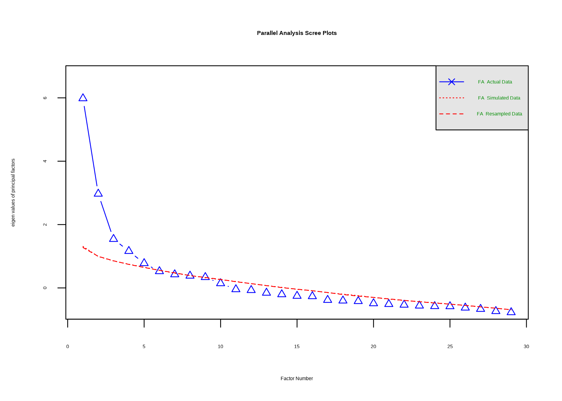
Parallel analysis suggests that the number of factors = 5 and the number of components = NA dat <- fa(Data, nfactors = lll[["nfact"]], rotate = "varimax", fm = "minres")
DD <- model_factors(data = dat, DATA = Data)
Loadings:
    MR1    MR2    MR3    MR5    MR4
x11  0.513  0.053  0.124  0.217  0.137
x12  0.611  0.127 -0.090  0.075  0.134
x13  0.559  0.354  0.115  0.020 -0.172
x20  0.556  0.049  0.083  0.306  0.059
x24  0.617 -0.284 -0.168  0.056  0.527
x25  0.718 -0.169  0.063  0.065  0.196
x26  0.595  0.048  0.104  0.205  0.139
x01  0.124  0.625 -0.077 -0.066  0.066
x02  0.039  0.783 -0.012  0.206  0.541
x10  0.254  0.631 -0.139  0.255 -0.081
x28 -0.086 -0.610  0.092  0.320  0.111
x04  0.239 -0.176  0.740 -0.101 -0.039
x05  0.149  0.065  0.792  0.074 -0.015
x06 -0.043 -0.260  0.720  0.157  0.186
x08 -0.130  0.016  0.594  0.255  0.452
x17  0.142 -0.192  0.044  0.667  0.137
x18  0.263  0.161 -0.041  0.527  0.073
x19  0.290  0.066  0.069  0.592  0.134
x03  0.087 -0.015  0.309  0.286  0.523
x07  0.302 -0.031  0.240  0.417  0.090
x09  0.112 -0.301  0.305  0.403  0.154
x14  0.345  0.153  0.203  0.203 -0.080
x15  0.480  0.275  0.262  0.069 -0.181
x16  0.125 -0.299  0.346  0.374  0.291
x21  0.492 -0.037  0.064  0.344 -0.065
x22  0.303 -0.238  0.039  0.286  0.481
x23  0.360 -0.440  0.021  0.207  0.499
x27         0.092  0.056         0.465
x29  0.216 -0.392  0.355  0.070  0.262

                 MR1   MR2   MR3   MR5   MR4
SS loadings    3.854 2.895 2.786 2.441 2.203
Proportion Var 0.133 0.100 0.096 0.084 0.076
Cumulative Var 0.133 0.233 0.329 0.413 0.489
DD$`Factors extracted`# A tibble: 29 × 6
Factor MR1 MR2 MR3 MR5 MR4
<chr> <dbl> <dbl> <dbl> <dbl> <dbl>
1 1 0.513 0 0 0 0
2 10 0 0.631 0 0 0
3 11 0 -0.61 0 0 0
4 12 0 0 0.74 0 0
5 13 0 0 0.792 0 0
6 14 0 0 0.72 0 0
7 15 0 0 0.594 0 0.452
8 16 0 0 0 0.667 0
9 17 0 0 0 0.527 0
10 18 0 0 0 0.592 0
# ℹ 19 more rowsDD$`factored data` MR1 MR2 MR3 MR5 MR4
1 19.292 -3.244 5.368 9.418 11.788
2 17.852 -2.068 5.368 9.015 11.788
3 17.804 1.711 5.368 6.892 11.788
4 19.292 -3.244 5.368 9.418 11.788
5 19.292 -3.244 5.368 8.826 11.788
6 19.292 -3.244 5.368 9.418 11.788
7 17.852 -3.244 4.628 7.434 12.253
8 19.292 -3.244 5.368 8.826 11.788
9 19.292 -3.244 5.368 8.826 11.788
10 17.852 -3.244 4.628 7.434 12.253
11 13.185 -2.083 4.180 6.183 7.375
12 12.867 -1.643 3.440 8.781 4.948
13 7.193 0.472 5.786 2.606 2.947
14 11.210 -1.643 2.846 2.606 4.919
15 9.629 -1.861 5.890 5.387 4.450
16 20.614 -2.963 4.378 3.725 9.963
17 11.499 -2.523 3.440 6.435 6.892
18 5.141 -0.811 2.846 2.606 2.947
19 7.193 -0.811 5.806 3.133 2.947
20 12.590 -2.502 7.912 6.852 6.892
21 20.885 0.470 14.230 10.550 14.933
22 22.114 0.300 13.438 10.035 16.941
23 19.346 1.503 14.230 10.086 14.520
24 13.861 0.438 5.870 6.764 11.766
25 16.868 1.476 3.586 8.162 11.684
26 11.735 0.098 5.066 6.236 9.722
27 20.465 2.733 10.018 7.812 10.087
28 13.972 0.708 7.694 7.570 10.626
29 22.698 0.300 12.916 11.559 14.497
30 14.522 0.463 10.882 7.887 10.632
31 23.309 0.252 12.124 12.613 15.519
32 22.708 0.300 12.718 12.438 15.426
33 16.808 -1.708 11.312 7.924 11.397
34 15.782 -0.458 11.312 7.924 12.327
35 16.808 -0.925 11.312 8.327 12.868
36 15.782 -1.708 11.312 7.924 11.397
37 15.782 -1.708 11.312 7.924 11.397
38 16.338 -2.100 11.312 7.924 11.397
39 13.827 -2.100 12.176 8.112 10.858
40 16.454 -1.660 11.312 7.924 12.882
41 15.782 -1.708 11.312 7.924 11.397
42 15.782 -0.925 11.312 7.924 11.938
43 11.057 -0.731 6.160 9.948 7.714
44 11.057 -0.731 6.160 9.948 7.714
45 12.518 -0.901 9.258 7.430 8.258
46 12.271 0.053 5.870 9.004 6.416
47 10.565 -0.949 4.920 8.724 6.852
48 11.057 -0.731 6.160 9.948 7.714
49 11.017 -0.339 7.620 8.711 8.121
50 13.945 -0.827 8.340 8.522 6.746
51 11.057 -0.731 6.160 9.142 7.714
52 12.103 -3.355 8.664 8.174 8.756
53 13.371 -2.502 7.172 7.475 7.822
54 13.383 -1.182 9.694 8.406 10.162
55 10.713 -1.182 9.100 7.475 7.694
56 11.141 -2.502 8.716 9.031 9.333
57 11.226 -1.182 7.172 5.894 6.790
58 12.106 -2.502 8.412 9.031 9.191
59 13.646 -2.502 9.476 9.031 9.814
60 12.149 -3.286 8.412 9.031 8.726
61 13.851 -2.502 13.636 8.439 11.199
62 14.263 -3.678 11.978 9.031 12.659
63 16.379 -2.439 9.476 8.471 8.319
64 13.591 -2.089 14.230 9.808 11.833
65 15.102 -3.292 14.230 10.642 11.709
66 20.424 -1.781 8.538 10.475 9.803
67 19.226 -1.580 9.998 8.536 8.358
68 11.690 -3.414 10.664 6.925 10.243
69 13.545 -0.811 4.628 5.568 9.722
70 16.446 -1.431 13.636 8.504 10.347
71 23.019 -3.663 9.944 11.836 14.283
72 18.596 -1.171 8.902 7.857 10.126
73 15.379 -2.238 7.224 8.211 8.858
74 12.999 -2.238 7.224 8.211 8.858
75 12.999 -2.238 7.224 8.211 8.858
76 14.763 -3.414 8.810 6.449 8.937
77 14.899 -1.628 5.838 6.449 10.456
78 18.292 -1.829 10.050 10.841 10.348
79 16.149 -1.781 9.258 7.527 7.857
80 18.245 -2.412 7.944 9.480 9.862
81 19.021 -2.852 7.818 9.897 10.348
82 17.677 -2.242 10.090 10.410 10.348
83 8.111 -0.557 6.734 11.179 4.450
84 18.296 -1.393 7.600 8.967 12.269
85 12.231 -2.068 11.384 6.605 8.419
86 14.079 -4.055 9.132 8.770 10.722
87 12.986 -1.989 6.466 6.686 5.320
88 13.523 -1.798 10.498 8.223 5.777
89 22.984 -4.686 8.110 8.554 11.965
90 11.049 -3.060 10.270 12.503 6.965
91 11.825 -2.083 11.998 7.448 8.837
92 13.245 -1.622 10.342 7.363 4.919
93 11.843 -2.364 10.196 5.879 6.421
94 15.614 -1.733 8.320 7.327 8.774
95 19.005 -3.286 8.464 7.605 11.788
96 17.447 -2.364 5.692 6.988 5.894
97 18.681 -1.580 5.692 6.988 6.948
98 15.614 -1.733 8.320 7.327 8.774
99 18.883 -1.733 5.692 6.018 7.870
100 16.185 -2.364 5.692 7.605 5.894
101 11.358 -2.295 5.672 8.851 4.345
102 14.111 -3.244 5.692 6.396 5.900
103 15.983 -2.364 5.692 6.018 6.483DD$`Factors list`$MR1
[1] 0.513 NA NA NA NA NA NA NA NA NA NA 0.611
[13] NA NA NA 0.480 NA 0.492 NA NA NA NA 0.559 0.556
[25] 0.617 0.718 0.595 NA NA
$MR2
[1] NA 0.631 NA NA NA NA NA NA NA NA NA NA
[13] NA NA NA NA NA NA NA NA NA NA NA NA
[25] NA NA NA 0.625 0.783
$MR3
[1] NA NA NA 0.740 0.792 0.720 0.594 NA NA NA NA NA
[13] NA NA NA NA NA NA NA NA NA NA NA NA
[25] NA NA NA NA NA
$MR5
[1] NA NA NA NA NA NA NA 0.667 0.527 0.592 NA NA
[13] 0.417 0.403 NA NA NA NA NA NA NA NA NA NA
[25] NA NA NA NA NA
$MR4
[1] NA NA NA NA NA NA 0.452 NA NA NA 0.523 NA
[13] NA NA NA NA NA NA 0.481 0.499 0.465 NA NA NA
[25] 0.527 NA NA NA 0.541DD$`Loadings data` Factor MR1 MR2 MR3 MR5 MR4
1 1 0.513 0.053 0.124 0.217 0.137
10 10 0.254 0.631 -0.139 0.255 -0.081
11 11 -0.086 -0.610 0.092 0.320 0.111
12 12 0.239 -0.176 0.740 -0.101 -0.039
13 13 0.149 0.065 0.792 0.074 -0.015
14 14 -0.043 -0.260 0.720 0.157 0.186
15 15 -0.130 0.016 0.594 0.255 0.452
16 16 0.142 -0.192 0.044 0.667 0.137
17 17 0.263 0.161 -0.041 0.527 0.073
18 18 0.290 0.066 0.069 0.592 0.134
19 19 0.087 -0.015 0.309 0.286 0.523
2 2 0.611 0.127 -0.090 0.075 0.134
20 20 0.302 -0.031 0.240 0.417 0.090
21 21 0.112 -0.301 0.305 0.403 0.154
22 22 0.345 0.153 0.203 0.203 -0.080
23 23 0.480 0.275 0.262 0.069 -0.181
24 24 0.125 -0.299 0.346 0.374 0.291
25 25 0.492 -0.037 0.064 0.344 -0.065
26 26 0.303 -0.238 0.039 0.286 0.481
27 27 0.360 -0.440 0.021 0.207 0.499
28 28 0.000 0.092 0.056 0.000 0.465
29 29 0.216 -0.392 0.355 0.070 0.262
3 3 0.559 0.354 0.115 0.020 -0.172
4 4 0.556 0.049 0.083 0.306 0.059
5 5 0.617 -0.284 -0.168 0.056 0.527
6 6 0.718 -0.169 0.063 0.065 0.196
7 7 0.595 0.048 0.104 0.205 0.139
8 8 0.124 0.625 -0.077 -0.066 0.066
9 9 0.039 0.783 -0.012 0.206 0.541DD$`Resilience capacity` [1] 0.4138058 0.4073301 0.4229417 0.4138058 0.4080583 0.4138058 0.3778932
[8] 0.4080583 0.4080583 0.3778932 0.2800000 0.2756602 0.1845049 0.1935728
[15] 0.2281068 0.3467670 0.2499320 0.1235825 0.1773592 0.3081942 0.5928932
[22] 0.6099806 0.5794660 0.3757184 0.4055922 0.3190000 0.4962621 0.3938835
[29] 0.6016505 0.4309320 0.6195825 0.6173786 0.4440097 0.4552136 0.4698058
[36] 0.4340485 0.4340485 0.4356408 0.4162427 0.4554563 0.4340485 0.4469029
[43] 0.3315340 0.3315340 0.3549806 0.3263495 0.2923495 0.3315340 0.3410680
[50] 0.3565631 0.3237087 0.3334175 0.3236699 0.3928447 0.3281553 0.3467864
[57] 0.2902913 0.3518252 0.3831553 0.3401165 0.4332330 0.4296408 0.3903495
[64] 0.4599320 0.4698155 0.4607670 0.4324078 0.3505631 0.3170097 0.4611845
[71] 0.5380485 0.4301942 0.3634369 0.3403301 0.3403301 0.3450971 0.3496505
[78] 0.4631262 0.3787379 0.4186311 0.4294369 0.4493495 0.2904563 0.4440680
[85] 0.3550583 0.3752233 0.2861068 0.3516796 0.4556019 0.3662816 0.3691748
[92] 0.3324951 0.3104369 0.3718641 0.4230680 0.3267670 0.3565922 0.3718641
[99] 0.3566019 0.3205049 0.2711748 0.2801456 0.3088544Welcome to the world of Data Science and easy Machine Learning!