Introduction
The advent of the COVID-19 pandemic really put everyone in confusion and as the days, weeks went-by, everyone was trying to understand the trend and the direction of the incidence. While the medicals were in their labs trying to understand the anatomy of the various, various statisticians and data scientists were trying to model the trend so as to guide future actions and preparations. One of the early models was done for Australia by (Krispin and Byrnes 2020). After observing the beatifuly animations of the incidence of the virus in the various regions of Australia, the motivation to do so was kindled. However, the first setback was the format the Nigerian Centre for Disease Control (NCDC) (NCDC 2020) was publishing the incidence in Nigeria was not very #RStats (R Core Team 2020) friendly. There were two main issues:
The data was and has been hard-formatted using the comma thousand separator which was and has remain difficult to easily analysed so alternative means of removing the format had to be worked out.
The data supplied by NCDC to the main collation centre of the COVID-19 at the Johns Hopkins University Center for Systems Science and Engineering (JHU-CCSE) (CCSE 2020) was not disaggregated by regions as in the case of Australia, therefore, the data had to be manualy compiled from the website (https://covid19.ncdc.gov.ng/) of the agency.
For the above two reasons, the animation for Nigeria could not be achieved almost immediately. After the initial manual compilation of the data set from NCDC, an animation of the incidence in Nigeria was made on the 3rd of May, 2020 as shown below.
Thereafter, daily summaries, trend of the observed cases and possible future path through modeling and forecasting were made once the data is updated. The forecast lenght was usually the total length of the observed data which entually led to the concept of equal length forecast. It was in this wise that it was observed that the changes in forecast with just a additional day’s data were quite alarming. Hence there was need to have a way of quickly comparing time-variant forecasts. After careful consideration, the concept was synthesized into the Dyn4cast package (Nmadu 2020). Presently, the package has five functions.
DynamicForecast
constrainedforecast
linearsystems
MLMetrics
MallowsCP
Percent
quicksummary
scaledlogit
invscaledlogit
The package is currently available in GitHub and can be installed as follows:
devtools::install_github("JobNmadu/Dyn4cast").
In this blog, the capabilities of the DynamicForecast function is explored.
Load the library and format the data
The sample data is the daily COVID-19 cases recorded and aggregagted into national data. The break points used for the splines modelling were established via visual examination of the observed data. The data cover the period 2020-02-29 to 2021-02-10.
library(Dyn4cast)
library(tidyverse)
data <- COVID19

data$Date <- as.Date(data$Date, format = '%m/%d/%Y')
date <- data$Date
series <- data$Case
Dss <- seq(data$Date[1], by = "day", length.out = length(data$Case))
lastdayfo21 <- Dss[length(Dss)]

BREAKS = c(70, 131, 173, 228, 274)
Modelling and forecast for the full data range
The constrained and unconstrained forecast are presented for compaison but the right one is the constrained forecast. It was necessary to consraine the forecast to the positive quadrant since ther is no zero and negative observations.
Days_full <- DynamicForecast(date = date, series = series, BREAKS = BREAKS, MaximumDate = "2021-02-10", Trend = "Day", Length = 0, Type = "Integer")
summary(Days_full$`Ensembled based on summed weight`)##
## Call:
## stats::lm(formula = Series ~ Without.knots + With.knots + Smooth +
## Quadratic + ARIMA)
##
## Residuals:
## Min 1Q Median 3Q Max
## -75.872 -13.916 5.702 20.586 26.472
##
## Coefficients:
## Estimate Std. Error t value Pr(>|t|)
## (Intercept) 32.437636 2.317418 13.997 <2e-16 ***
## Without.knots -0.027043 0.016919 -1.598 0.111
## With.knots -0.002837 0.018257 -0.155 0.877
## Smooth -0.009017 0.015934 -0.566 0.572
## Quadratic 0.368732 0.007405 49.797 <2e-16 ***
## ARIMA 0.010110 0.015349 0.659 0.511
## ---
## Signif. codes: 0 '***' 0.001 '**' 0.01 '*' 0.05 '.' 0.1 ' ' 1
##
## Residual standard error: 24.41 on 342 degrees of freedom
## Multiple R-squared: 0.942, Adjusted R-squared: 0.9412
## F-statistic: 1111 on 5 and 342 DF, p-value: < 2.2e-16knitr::kable(as.data.frame(Days_full$`Unconstrained Forecast`),
row.names = FALSE, "html")| DDf91 | Case |
|---|---|
| Linear | 462222 |
| Semilog | 261819 |
| Growth | 3158 |
| Without knots | 2252100 |
| Smooth Spline | 2585104 |
| With knots | -1885886 |
| Quadratic Polynomial | 700873 |
| Lower ARIMA | -275249 |
| Upper ARIMA | 945658 |
| Essembled with equal weight | 464539 |
| Essembled based on weight | 181673 |
| Essembled based on summed weight | 208354 |
| Essembled based on weight of fit | 414914 |
knitr::kable(as.data.frame(Days_full$`Constrained Forecast`),
row.names = FALSE, "html")| Model | Confirmed cases |
|---|---|
| Linear | 462222 |
| Semilog | 261819 |
| Growth | 3158 |
| Without knots 80% | 126351 |
| Without knots 95% | 682497 |
| Smooth Spline 80% | 494904 |
| Smooth Spline 95% | 841141 |
| With knots 80% | 446278 |
| With knots 95% | 818931 |
| Quadratic Polynomial 80% | 656466 |
| Quadratic Polynomial 95% | 692625 |
| ARIMA 80% | 22070 |
| ARIMA 95% | 925882 |
| Essembled with equal weight 80% | 179428 |
| Essembled with equal weight 95% | 844147 |
| Essembled based on weight 80% | 88055 |
| Essembled based on weight 95% | 200922 |
| Essembled based on summed weight 80% | 94099 |
| Essembled based on summed weight 95% | 553710 |
| Essembled based on weight of fit 80% | 64139 |
| Essembled based on weight of fit 95% | 907909 |
knitr::kable(as.data.frame(Days_full$RMSE), row.names = FALSE, "html")| DDf91 | RMSE_f91 |
|---|---|
| Linear | 369.14 |
| Semilog | 397.82 |
| Growth | 612.54 |
| Without knots | 268.34 |
| Smooth Spline | 255.21 |
| With knots | 189.71 |
| Quadratic Polynomial | 351.21 |
| Lower ARIMA | 210.57 |
| Upper ARIMA | 210.57 |
| Essembled with equal weight | 226.04 |
| Essembled based on weight | 471.12 |
| Essembled based on summed weight | 470.5 |
| Essembled based on weight of fit | 285.48 |
Days_full$`Unconstrained forecast Plot`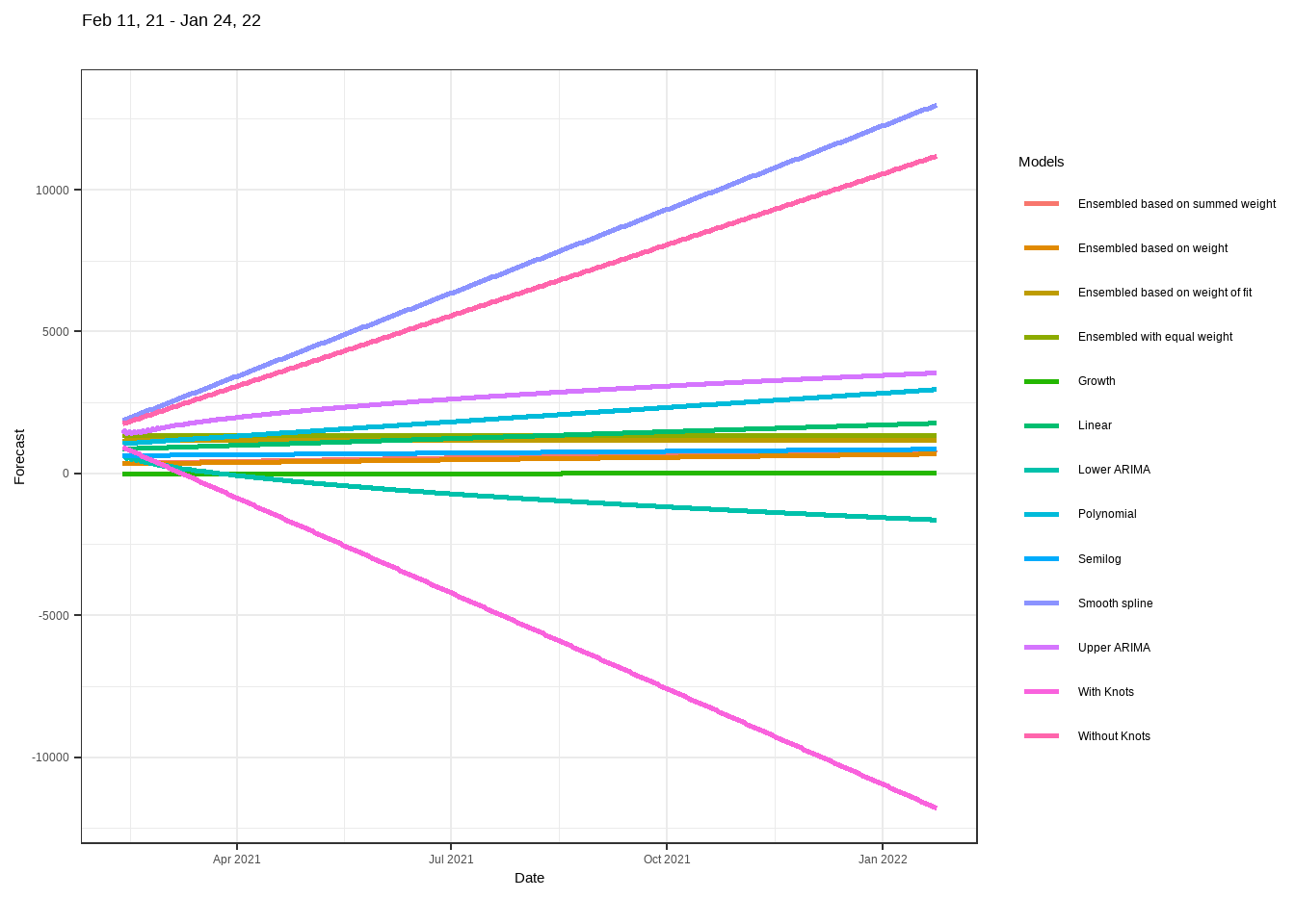
Days_full$`Constrained forecast Plot`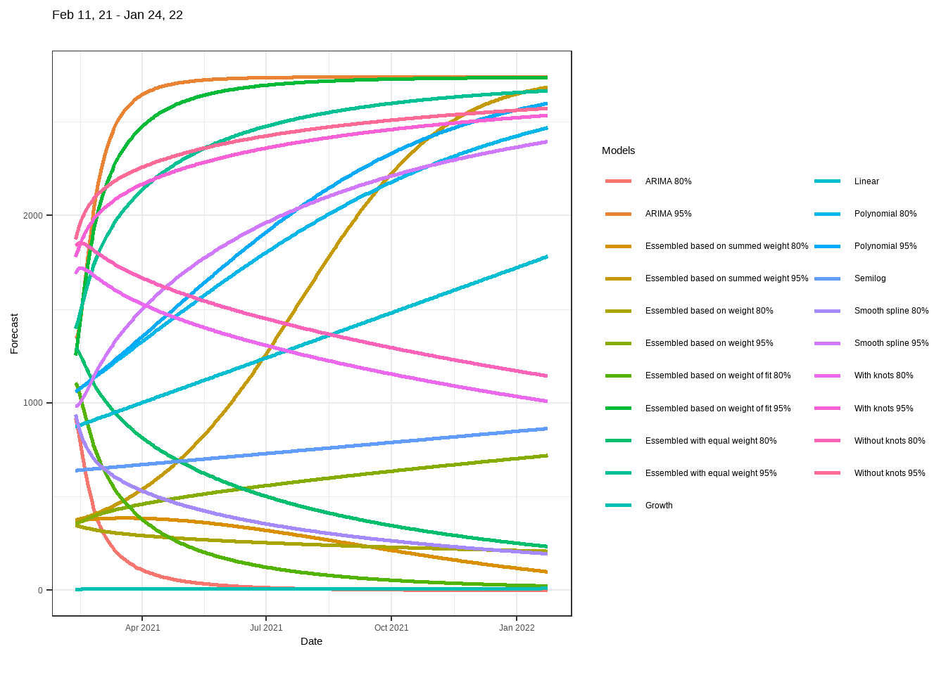
Modelling and forecast by using data as at 28 days earlier
KK_28 <- data[data$Date <= lastdayfo21 - 28, ]
date <- KK_28$Date
series <- KK_28$Case
Days_28 <- DynamicForecast(date = date, series = series, BREAKS = BREAKS, MaximumDate = "2021-02-10", Trend = "Day", Length = 0, Type = "Integer")## Model matrix is rank deficient. Parameters `x` were not estimable.
## Model matrix is rank deficient. Parameters `x` were not estimable.
## Model matrix is rank deficient. Parameters `x` were not estimable.
## Model matrix is rank deficient. Parameters `x` were not estimable.
## Model matrix is rank deficient. Parameters `x` were not estimable.
## Model matrix is rank deficient. Parameters `x` were not estimable.summary(Days_28$`Ensembled based on summed weight`)##
## Call:
## stats::lm(formula = Series ~ Without.knots + With.knots + Smooth +
## Quadratic + ARIMA)
##
## Residuals:
## Min 1Q Median 3Q Max
## -57.604 -15.834 6.197 20.574 27.660
##
## Coefficients:
## Estimate Std. Error t value Pr(>|t|)
## (Intercept) -28.863297 3.022289 -9.550 <2e-16 ***
## Without.knots 0.003672 0.012301 0.298 0.7655
## With.knots 0.001627 0.017763 0.092 0.9271
## Smooth -0.030868 0.020663 -1.494 0.1362
## Quadratic 0.564357 0.010223 55.204 <2e-16 ***
## ARIMA 0.028727 0.013946 2.060 0.0402 *
## ---
## Signif. codes: 0 '***' 0.001 '**' 0.01 '*' 0.05 '.' 0.1 ' ' 1
##
## Residual standard error: 23.09 on 314 degrees of freedom
## Multiple R-squared: 0.9387, Adjusted R-squared: 0.9377
## F-statistic: 961.9 on 5 and 314 DF, p-value: < 2.2e-16knitr::kable(as.data.frame(Days_28$`Unconstrained Forecast`),
row.names = FALSE, "html")| DDf91 | Case |
|---|---|
| Linear | 277722 |
| Semilog | 179540 |
| Growth | 2721 |
| Without knots | 1606956 |
| Smooth Spline | 2082046 |
| With knots | 991316 |
| Quadratic Polynomial | 389104 |
| Lower ARIMA | -126404 |
| Upper ARIMA | 939766 |
| Essembled with equal weight | 1405086 |
| Essembled based on weight | 153744 |
| Essembled based on summed weight | 217150 |
| Essembled based on weight of fit | 1101861 |
knitr::kable(as.data.frame(Days_28$`Constrained Forecast`),
row.names = FALSE, "html")| Model | Confirmed cases |
|---|---|
| Linear | 277722 |
| Semilog | 179540 |
| Growth | 2721 |
| Without knots 80% | 187609 |
| Without knots 95% | 782270 |
| Smooth Spline 80% | 13054 |
| Smooth Spline 95% | 871070 |
| With knots 80% | 235264 |
| With knots 95% | 678456 |
| Quadratic Polynomial 80% | 414340 |
| Quadratic Polynomial 95% | 441909 |
| ARIMA 80% | 86426 |
| ARIMA 95% | 847342 |
| Essembled with equal weight 80% | 148671 |
| Essembled with equal weight 95% | 775984 |
| Essembled based on weight 80% | 73488 |
| Essembled based on weight 95% | 174024 |
| Essembled based on summed weight 80% | 217138 |
| Essembled based on summed weight 95% | 386468 |
| Essembled based on weight of fit 80% | 152548 |
| Essembled based on weight of fit 95% | 669194 |
knitr::kable(as.data.frame(Days_28$RMSE), row.names = FALSE, "html")| DDf91 | RMSE_f91 |
|---|---|
| Linear | 307.33 |
| Semilog | 310.78 |
| Growth | 475.6 |
| Without knots | 221.72 |
| Smooth Spline | 185.4 |
| With knots | 153.91 |
| Quadratic Polynomial | 305.23 |
| Lower ARIMA | 169.16 |
| Upper ARIMA | 169.16 |
| Essembled with equal weight | 178.28 |
| Essembled based on weight | 358.35 |
| Essembled based on summed weight | 357.47 |
| Essembled based on weight of fit | 193.38 |
Days_28$`Unconstrained forecast Plot`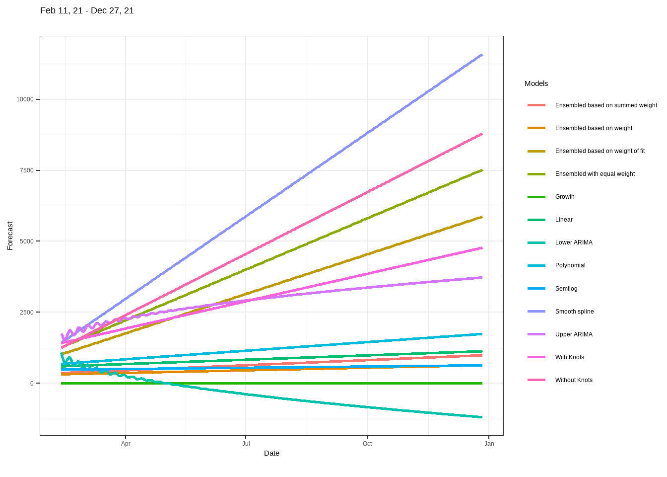
Days_28$`Constrained forecast Plot`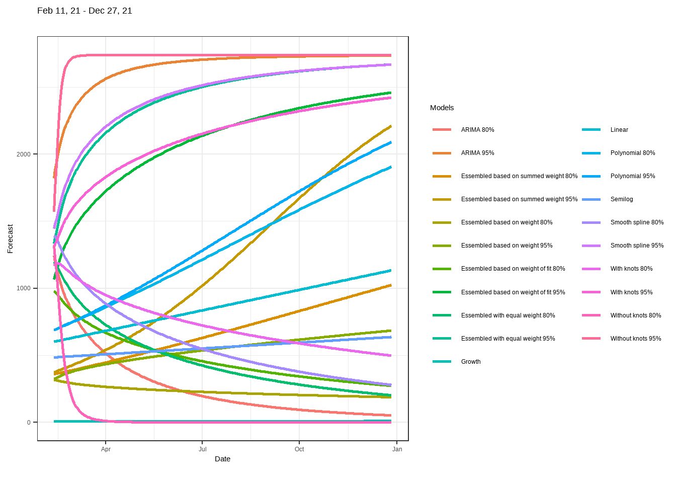
Modelling and forecast by using data as at 14 days earlier
KK_14 <- data[data$Date <= lastdayfo21 - 14, ]
date <- KK_14$Date
series <- KK_14$Case

Days_14 <- DynamicForecast(date = date, series = series, BREAKS = BREAKS, MaximumDate = "2021-02-10", Trend = "Day", Length = 0, Type = "Integer")## Model matrix is rank deficient. Parameters `x` were not estimable.
## Model matrix is rank deficient. Parameters `x` were not estimable.
## Model matrix is rank deficient. Parameters `x` were not estimable.
## Model matrix is rank deficient. Parameters `x` were not estimable.
## Model matrix is rank deficient. Parameters `x` were not estimable.
## Model matrix is rank deficient. Parameters `x` were not estimable.summary(Days_14$`Ensembled based on weight`)##
## Call:
## stats::lm(formula = Series ~ Without.knots * With.knots * Smooth *
## Quadratic * ARIMA)
##
## Residuals:
## Min 1Q Median 3Q Max
## -0.195806 -0.029597 -0.002006 0.030330 0.166867
##
## Coefficients:
## Estimate Std. Error t value
## (Intercept) -3.868e+01 5.590e-02 -691.851
## Without.knots 1.886e-01 2.398e-04 786.281
## With.knots -7.224e-02 3.401e-04 -212.394
## Smooth -3.557e-02 4.413e-03 -8.059
## Quadratic 5.811e-01 2.470e-04 2352.470
## ARIMA 1.885e-02 2.666e-03 7.073
## Without.knots:With.knots -4.036e-06 7.296e-07 -5.531
## Without.knots:Smooth 1.640e-04 1.933e-05 8.486
## With.knots:Smooth -7.377e-05 1.009e-05 -7.314
## Without.knots:Quadratic -1.145e-03 1.715e-06 -667.288
## With.knots:Quadratic 8.529e-04 2.021e-06 422.038
## Smooth:Quadratic 7.659e-05 9.532e-06 8.035
## Without.knots:ARIMA -1.038e-04 1.079e-05 -9.620
## With.knots:ARIMA 6.844e-05 5.947e-06 11.508
## Smooth:ARIMA 2.718e-04 5.914e-05 4.596
## Quadratic:ARIMA -3.738e-05 5.949e-06 -6.284
## Without.knots:With.knots:Smooth -3.987e-08 4.727e-09 -8.434
## Without.knots:With.knots:Quadratic -6.362e-09 1.129e-09 -5.634
## Without.knots:Smooth:Quadratic -5.393e-07 5.896e-08 -9.146
## With.knots:Smooth:Quadratic 4.136e-07 4.369e-08 9.467
## Without.knots:With.knots:ARIMA -1.048e-08 4.833e-09 -2.168
## Without.knots:Smooth:ARIMA -1.160e-06 2.292e-07 -5.059
## With.knots:Smooth:ARIMA 5.780e-07 1.119e-07 5.165
## Without.knots:Quadratic:ARIMA 2.415e-07 3.506e-08 6.889
## With.knots:Quadratic:ARIMA -1.811e-07 2.694e-08 -6.721
## Smooth:Quadratic:ARIMA -5.914e-07 1.279e-07 -4.622
## Without.knots:With.knots:Smooth:Quadratic 3.038e-11 4.052e-12 7.497
## Without.knots:With.knots:Smooth:ARIMA 8.924e-11 7.261e-12 12.289
## Without.knots:With.knots:Quadratic:ARIMA 1.143e-11 4.224e-12 2.706
## Without.knots:Smooth:Quadratic:ARIMA 3.719e-09 7.437e-10 5.001
## With.knots:Smooth:Quadratic:ARIMA -2.796e-09 5.474e-10 -5.109
## Without.knots:With.knots:Smooth:Quadratic:ARIMA -5.143e-14 3.878e-15 -13.264
## Pr(>|t|)
## (Intercept) < 2e-16 ***
## Without.knots < 2e-16 ***
## With.knots < 2e-16 ***
## Smooth 1.81e-14 ***
## Quadratic < 2e-16 ***
## ARIMA 1.06e-11 ***
## Without.knots:With.knots 6.90e-08 ***
## Without.knots:Smooth 9.74e-16 ***
## With.knots:Smooth 2.34e-12 ***
## Without.knots:Quadratic < 2e-16 ***
## With.knots:Quadratic < 2e-16 ***
## Smooth:Quadratic 2.12e-14 ***
## Without.knots:ARIMA < 2e-16 ***
## With.knots:ARIMA < 2e-16 ***
## Smooth:ARIMA 6.35e-06 ***
## Quadratic:ARIMA 1.15e-09 ***
## Without.knots:With.knots:Smooth 1.40e-15 ***
## Without.knots:With.knots:Quadratic 4.03e-08 ***
## Without.knots:Smooth:Quadratic < 2e-16 ***
## With.knots:Smooth:Quadratic < 2e-16 ***
## Without.knots:With.knots:ARIMA 0.0309 *
## Without.knots:Smooth:ARIMA 7.33e-07 ***
## With.knots:Smooth:ARIMA 4.37e-07 ***
## Without.knots:Quadratic:ARIMA 3.28e-11 ***
## With.knots:Quadratic:ARIMA 8.98e-11 ***
## Smooth:Quadratic:ARIMA 5.63e-06 ***
## Without.knots:With.knots:Smooth:Quadratic 7.33e-13 ***
## Without.knots:With.knots:Smooth:ARIMA < 2e-16 ***
## Without.knots:With.knots:Quadratic:ARIMA 0.0072 **
## Without.knots:Smooth:Quadratic:ARIMA 9.68e-07 ***
## With.knots:Smooth:Quadratic:ARIMA 5.76e-07 ***
## Without.knots:With.knots:Smooth:Quadratic:ARIMA < 2e-16 ***
## ---
## Signif. codes: 0 '***' 0.001 '**' 0.01 '*' 0.05 '.' 0.1 ' ' 1
##
## Residual standard error: 0.0534 on 302 degrees of freedom
## Multiple R-squared: 1, Adjusted R-squared: 1
## F-statistic: 3.512e+07 on 31 and 302 DF, p-value: < 2.2e-16knitr::kable(as.data.frame(Days_14$`Unconstrained Forecast`),
row.names = FALSE, "html")| DDf91 | Case |
|---|---|
| Linear | 393218 |
| Semilog | 195751 |
| Growth | 2962 |
| Without knots | 2257939 |
| Smooth Spline | 2732835 |
| With knots | 1080847 |
| Quadratic Polynomial | 592450 |
| Lower ARIMA | 341460 |
| Upper ARIMA | 1286528 |
| Essembled with equal weight | 1567506 |
| Essembled based on weight | 167500 |
| Essembled based on summed weight | 193050 |
| Essembled based on weight of fit | 1238616 |
knitr::kable(as.data.frame(Days_14$`Constrained Forecast`),
row.names = FALSE, "html")| Model | Confirmed cases |
|---|---|
| Linear | 393218 |
| Semilog | 195751 |
| Growth | 2962 |
| Without knots 80% | 34305 |
| Without knots 95% | NaN |
| Smooth Spline 80% | 345858 |
| Smooth Spline 95% | 865177 |
| With knots 80% | 197708 |
| With knots 95% | 865132 |
| Quadratic Polynomial 80% | 578610 |
| Quadratic Polynomial 95% | 615408 |
| ARIMA 80% | 117721 |
| ARIMA 95% | 881259 |
| Essembled with equal weight 80% | 122650 |
| Essembled with equal weight 95% | 885542 |
| Essembled based on weight 80% | 51428 |
| Essembled based on weight 95% | 340684 |
| Essembled based on summed weight 80% | 125985 |
| Essembled based on summed weight 95% | 462276 |
| Essembled based on weight of fit 80% | 13542 |
| Essembled based on weight of fit 95% | 909625 |
knitr::kable(as.data.frame(Days_14$RMSE), row.names = FALSE, "html")| DDf91 | RMSE_f91 |
|---|---|
| Linear | 359.04 |
| Semilog | 379.11 |
| Growth | 570.94 |
| Without knots | 231.2 |
| Smooth Spline | 197.7 |
| With knots | 130.1 |
| Quadratic Polynomial | 345.1 |
| Lower ARIMA | 186.95 |
| Upper ARIMA | 186.95 |
| Essembled with equal weight | 185.12 |
| Essembled based on weight | 440.75 |
| Essembled based on summed weight | 440.29 |
| Essembled based on weight of fit | 258.59 |
Days_14$`Unconstrained forecast Plot`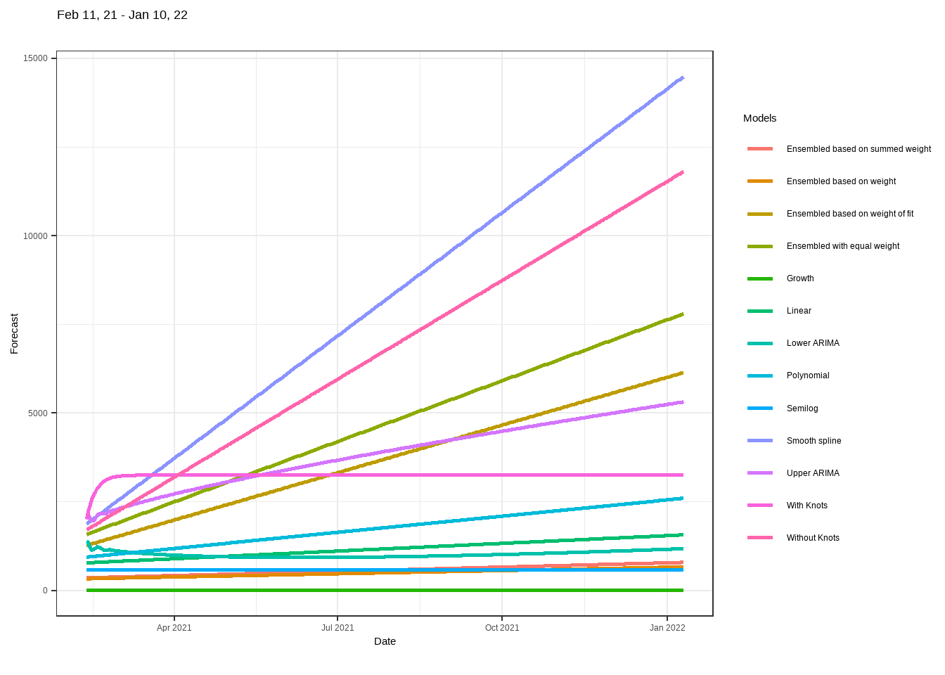
Days_14$`Constrained forecast Plot`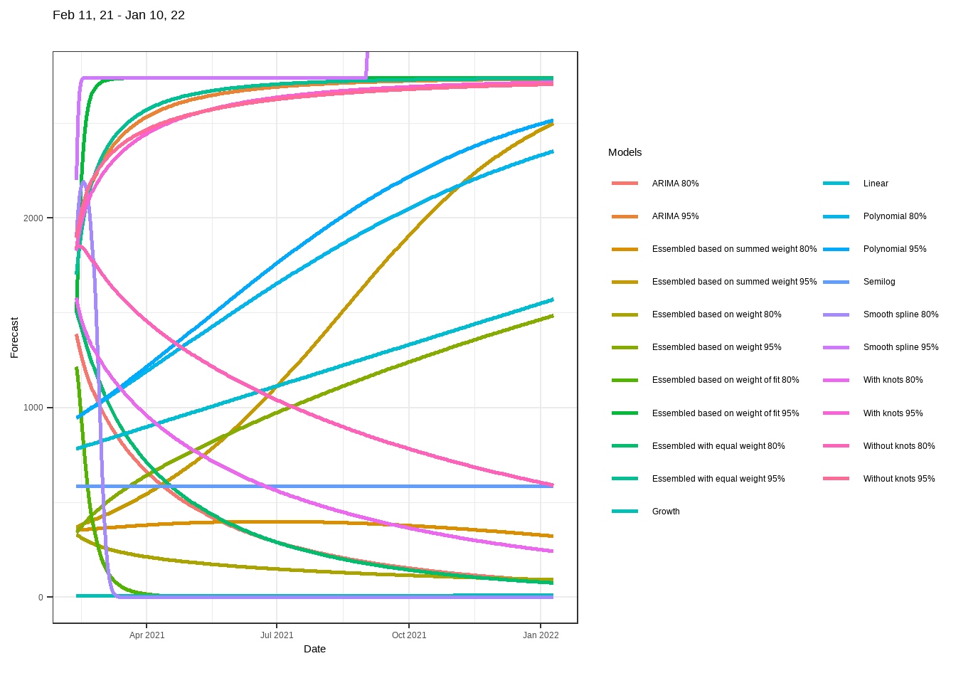
Modelling and forecast by using data as at 1 day earlier
KK_1 <- data[data$Date <= lastdayfo21 - 1, ]
date <- KK_1$Date
series <- KK_1$Case

Days_1 <- DynamicForecast(date = date, series = series, BREAKS = BREAKS, MaximumDate = "2021-02-10", Trend = "Day", Length = 0, Type = "Integer")## Model matrix is rank deficient. Parameters `x` were not estimable.
## Model matrix is rank deficient. Parameters `x` were not estimable.
## Model matrix is rank deficient. Parameters `x` were not estimable.
## Model matrix is rank deficient. Parameters `x` were not estimable.
## Model matrix is rank deficient. Parameters `x` were not estimable.
## Model matrix is rank deficient. Parameters `x` were not estimable.summary(Days_1$`Ensembled based on weight`)##
## Call:
## stats::lm(formula = Series ~ Without.knots * With.knots * Smooth *
## Quadratic * ARIMA)
##
## Residuals:
## Min 1Q Median 3Q Max
## -0.21373 -0.03116 -0.00320 0.02753 0.18117
##
## Coefficients:
## Estimate Std. Error t value
## (Intercept) -2.920e+01 5.290e-02 -551.900
## Without.knots 2.011e-01 3.346e-04 601.061
## With.knots -7.955e-02 6.473e-04 -122.896
## Smooth -6.038e-02 9.399e-03 -6.424
## Quadratic 5.297e-01 3.614e-04 1465.793
## ARIMA -3.211e-02 5.951e-03 -5.395
## Without.knots:With.knots -6.730e-06 1.417e-06 -4.750
## Without.knots:Smooth 3.472e-04 5.077e-05 6.838
## With.knots:Smooth -1.636e-04 2.999e-05 -5.456
## Without.knots:Quadratic -1.301e-03 2.970e-06 -438.139
## With.knots:Quadratic 1.048e-03 3.966e-06 264.346
## Smooth:Quadratic 9.837e-05 1.742e-05 5.646
## Without.knots:ARIMA 9.806e-05 3.785e-05 2.591
## With.knots:ARIMA -1.637e-05 2.322e-05 -0.705
## Smooth:ARIMA 5.924e-04 1.581e-04 3.747
## Quadratic:ARIMA 6.050e-05 1.041e-05 5.813
## Without.knots:With.knots:Smooth -9.628e-08 1.617e-08 -5.953
## Without.knots:With.knots:Quadratic -9.005e-09 1.211e-09 -7.439
## Without.knots:Smooth:Quadratic -1.016e-06 1.487e-07 -6.830
## With.knots:Smooth:Quadratic 8.247e-07 1.203e-07 6.857
## Without.knots:With.knots:ARIMA -1.536e-08 1.107e-08 -1.388
## Without.knots:Smooth:ARIMA -3.010e-06 7.324e-07 -4.110
## With.knots:Smooth:ARIMA 1.579e-06 3.796e-07 4.161
## Without.knots:Quadratic:ARIMA -4.196e-07 9.617e-08 -4.363
## With.knots:Quadratic:ARIMA 3.042e-07 7.743e-08 3.928
## Smooth:Quadratic:ARIMA -1.053e-06 2.870e-07 -3.669
## Without.knots:With.knots:Smooth:Quadratic 6.621e-11 1.370e-11 4.832
## Without.knots:With.knots:Smooth:ARIMA 2.534e-10 4.002e-11 6.332
## Without.knots:With.knots:Quadratic:ARIMA 1.809e-11 7.723e-12 2.343
## Without.knots:Smooth:Quadratic:ARIMA 8.974e-09 2.242e-09 4.002
## With.knots:Smooth:Quadratic:ARIMA -7.160e-09 1.763e-09 -4.061
## Without.knots:With.knots:Smooth:Quadratic:ARIMA -1.367e-13 2.744e-14 -4.983
## Pr(>|t|)
## (Intercept) < 2e-16 ***
## Without.knots < 2e-16 ***
## With.knots < 2e-16 ***
## Smooth 4.89e-10 ***
## Quadratic < 2e-16 ***
## ARIMA 1.35e-07 ***
## Without.knots:With.knots 3.10e-06 ***
## Without.knots:Smooth 4.17e-11 ***
## With.knots:Smooth 9.88e-08 ***
## Without.knots:Quadratic < 2e-16 ***
## With.knots:Quadratic < 2e-16 ***
## Smooth:Quadratic 3.66e-08 ***
## Without.knots:ARIMA 0.010024 *
## With.knots:ARIMA 0.481343
## Smooth:ARIMA 0.000213 ***
## Quadratic:ARIMA 1.50e-08 ***
## Without.knots:With.knots:Smooth 7.00e-09 ***
## Without.knots:With.knots:Quadratic 9.74e-13 ***
## Without.knots:Smooth:Quadratic 4.37e-11 ***
## With.knots:Smooth:Quadratic 3.73e-11 ***
## Without.knots:With.knots:ARIMA 0.166164
## Without.knots:Smooth:ARIMA 5.05e-05 ***
## With.knots:Smooth:ARIMA 4.10e-05 ***
## Without.knots:Quadratic:ARIMA 1.74e-05 ***
## With.knots:Quadratic:ARIMA 0.000105 ***
## Smooth:Quadratic:ARIMA 0.000286 ***
## Without.knots:With.knots:Smooth:Quadratic 2.12e-06 ***
## Without.knots:With.knots:Smooth:ARIMA 8.34e-10 ***
## Without.knots:With.knots:Quadratic:ARIMA 0.019753 *
## Without.knots:Smooth:Quadratic:ARIMA 7.83e-05 ***
## With.knots:Smooth:Quadratic:ARIMA 6.18e-05 ***
## Without.knots:With.knots:Smooth:Quadratic:ARIMA 1.03e-06 ***
## ---
## Signif. codes: 0 '***' 0.001 '**' 0.01 '*' 0.05 '.' 0.1 ' ' 1
##
## Residual standard error: 0.05177 on 315 degrees of freedom
## Multiple R-squared: 1, Adjusted R-squared: 1
## F-statistic: 4.191e+07 on 31 and 315 DF, p-value: < 2.2e-16knitr::kable(as.data.frame(Days_1$`Unconstrained Forecast`),
row.names = FALSE, "html")| DDf91 | Case |
|---|---|
| Linear | 457715 |
| Semilog | 221661 |
| Growth | 3144 |
| Without knots | 2257880 |
| Smooth Spline | 2601172 |
| With knots | -2249595 |
| Quadratic Polynomial | 694018 |
| Lower ARIMA | -178192 |
| Upper ARIMA | 912705 |
| Essembled with equal weight | 424188 |
| Essembled based on weight | 180150 |
| Essembled based on summed weight | 185853 |
| Essembled based on weight of fit | 383239 |
knitr::kable(as.data.frame(Days_1$`Constrained Forecast`),
row.names = FALSE, "html")| Model | Confirmed cases |
|---|---|
| Linear | 457715 |
| Semilog | 221661 |
| Growth | 3144 |
| Without knots 80% | 54481 |
| Without knots 95% | 820859 |
| Smooth Spline 80% | 15966 |
| Smooth Spline 95% | 948126 |
| With knots 80% | 32428 |
| With knots 95% | 944351 |
| Quadratic Polynomial 80% | 651633 |
| Quadratic Polynomial 95% | 687875 |
| ARIMA 80% | 47155 |
| ARIMA 95% | 907522 |
| Essembled with equal weight 80% | 92279 |
| Essembled with equal weight 95% | 895305 |
| Essembled based on weight 80% | 85678 |
| Essembled based on weight 95% | 205673 |
| Essembled based on summed weight 80% | 98217 |
| Essembled based on summed weight 95% | 479362 |
| Essembled based on weight of fit 80% | 191518 |
| Essembled based on weight of fit 95% | 739663 |
knitr::kable(as.data.frame(Days_1$RMSE), row.names = FALSE, "html")| DDf91 | RMSE_f91 |
|---|---|
| Linear | 369.41 |
| Semilog | 397.51 |
| Growth | 610.45 |
| Without knots | 266.74 |
| Smooth Spline | 252.65 |
| With knots | 189.7 |
| Quadratic Polynomial | 351.7 |
| Lower ARIMA | 210.45 |
| Upper ARIMA | 210.45 |
| Essembled with equal weight | 225.41 |
| Essembled based on weight | 469.93 |
| Essembled based on summed weight | 469.3 |
| Essembled based on weight of fit | 283.82 |
Days_1$`Unconstrained forecast Plot`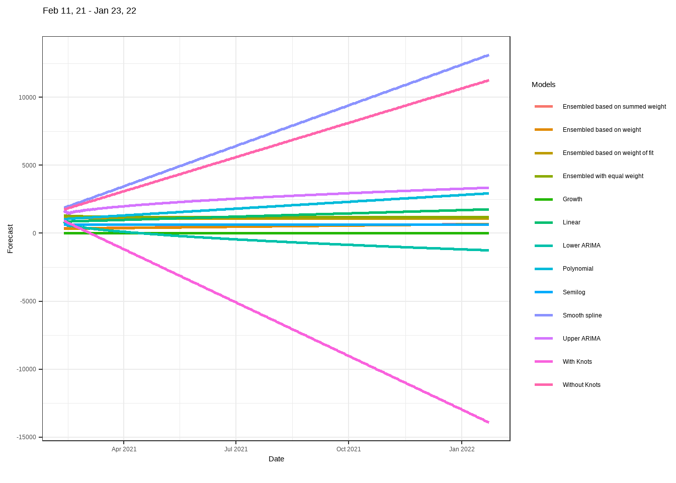
Days_1$`Constrained forecast Plot`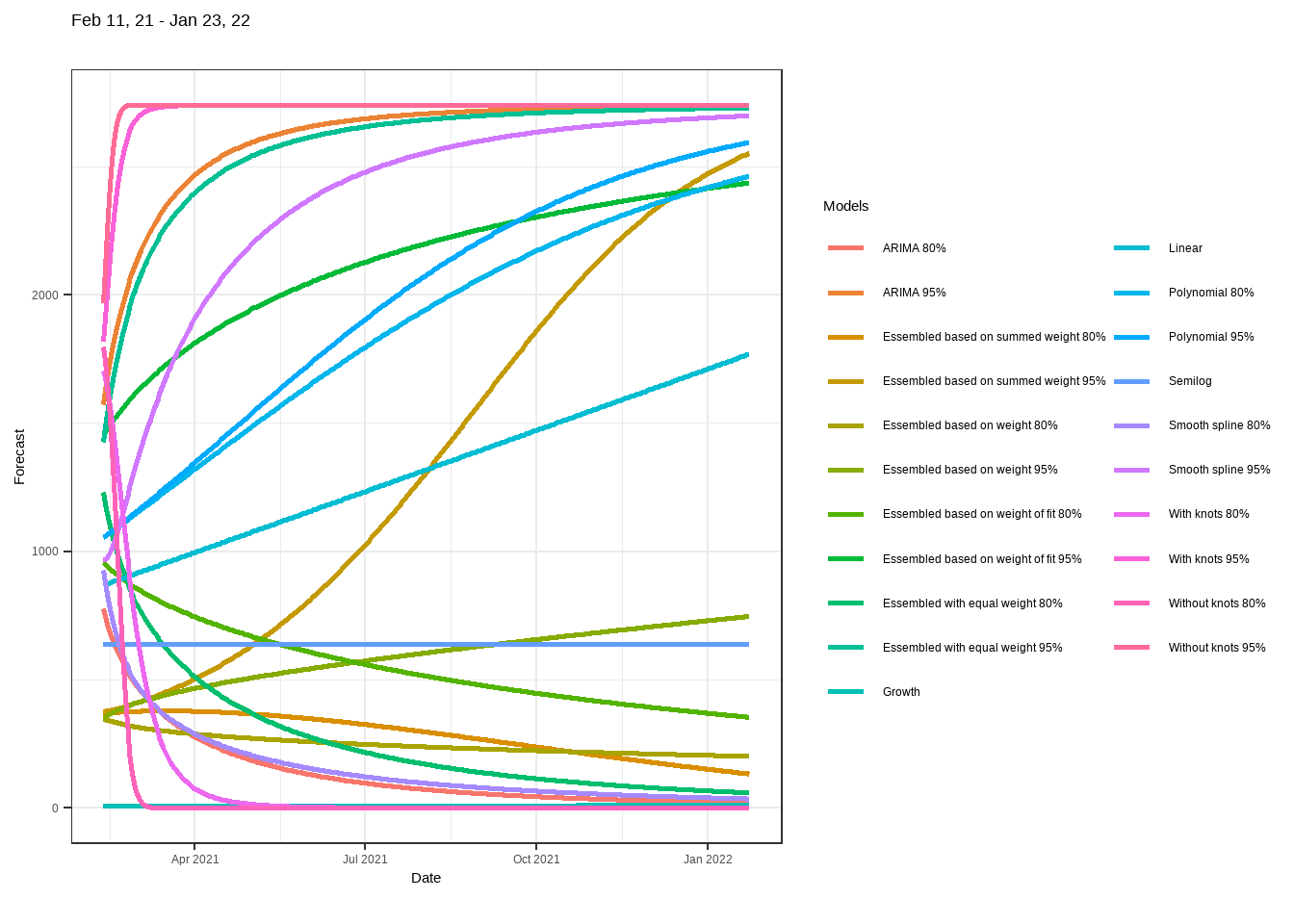
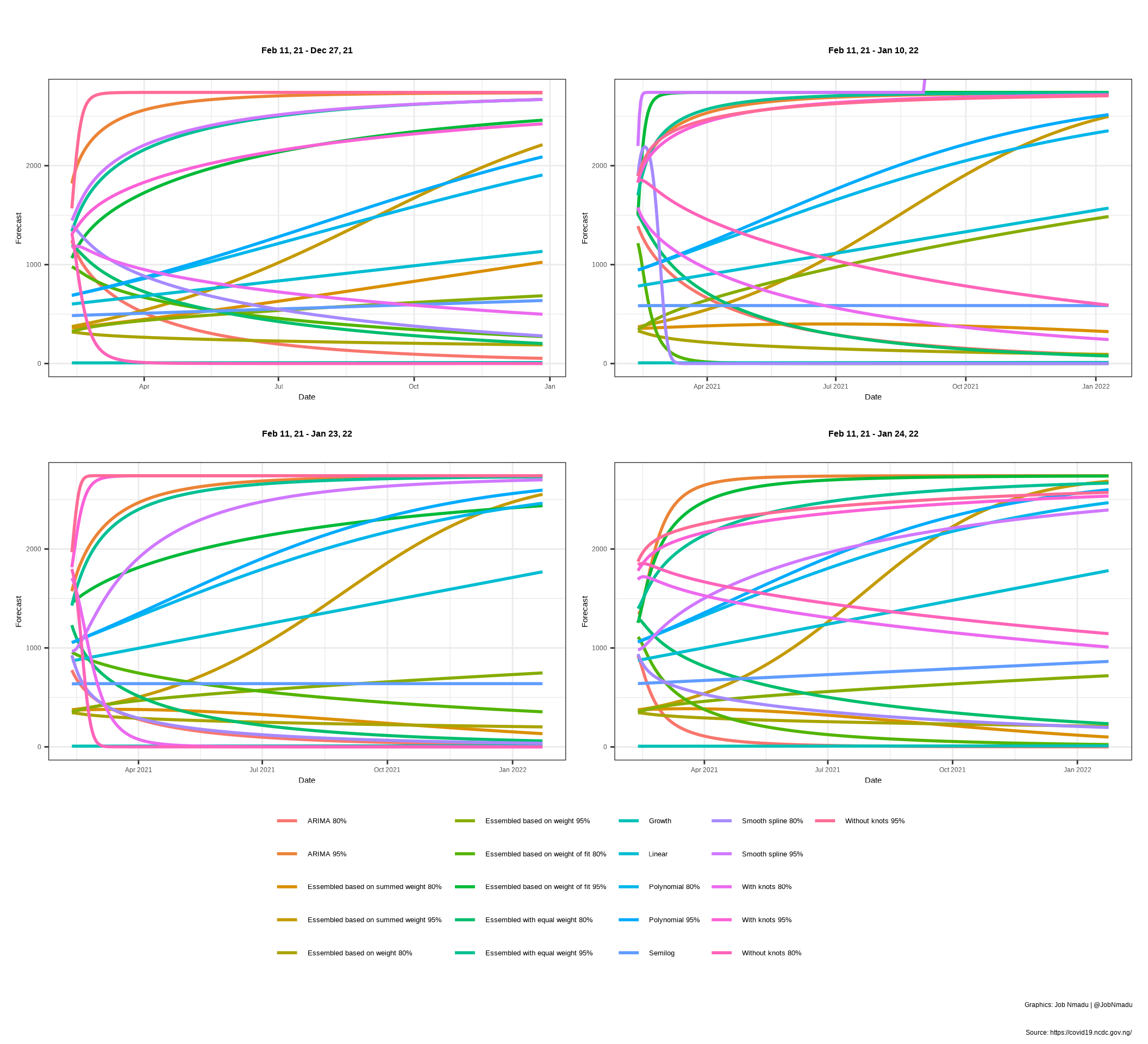
Comparing the constrained forecast plots for the four-time periods